Comparing Alignment Methods

Introduction

fdars provides four approaches to curve alignment, each with different trade-offs in terms of automation, smoothness, interpretability, and speed. This article compares them side-by-side on the same data, and provides guidance on when to use each method.

The four methods are:

Elastic alignment (elastic.align, karcher.mean) – global optimization via dynamic programming in SRSF space. See vignette("elastic-alignment", package = "fdars") for full details.
Landmark registration (landmark.register) – feature-based piecewise-linear warping. See vignette("landmark-registration", package = "fdars") for full details.
Constrained elastic alignment (elastic.align.constrained) – elastic alignment with landmark pass-through constraints
TSRVF (tsrvf.transform) – not an alignment method per se, but a linearization of elastic alignment for downstream analysis. See vignette("tsrvf", package = "fdars") for full details.

library(fdars)
#> 
#> Attaching package: 'fdars'
#> The following objects are masked from 'package:stats':
#> 
#>     cov, decompose, deriv, median, sd, var
#> The following object is masked from 'package:base':
#> 
#>     norm
library(ggplot2)
library(patchwork)
theme_set(theme_minimal())

Test Data

We use two datasets that highlight different alignment challenges.

Dataset 1: Smooth Phase Shifts

Curves with smooth, global timing differences – the classic alignment scenario:

set.seed(42)
argvals <- seq(0, 1, length.out = 200)
n <- 15

data_smooth <- matrix(0, n, 200)
for (i in 1:n) {
  shift <- runif(1, -0.1, 0.1)
  amp <- rnorm(1, 1, 0.15)
  data_smooth[i, ] <- amp * sin(2 * pi * (argvals - shift)) +
                       0.4 * amp * sin(4 * pi * (argvals - shift * 0.7))
}
fd_smooth <- fdata(data_smooth, argvals = argvals)

Dataset 2: Distinct Feature Shifts

Curves with clearly identifiable peaks that shift independently – where domain knowledge matters:

data_feat <- matrix(0, n, 200)
for (i in 1:n) {
  pk1 <- runif(1, 0.15, 0.35)
  pk2 <- runif(1, 0.55, 0.75)
  w1 <- rnorm(1, 1, 0.2)
  w2 <- rnorm(1, 0.8, 0.15)
  data_feat[i, ] <- w1 * exp(-200 * (argvals - pk1)^2) +
                     w2 * exp(-200 * (argvals - pk2)^2) +
                     0.05 * rnorm(200)
}
fd_feat <- fdata(data_feat, argvals = argvals)

p1 <- plot(fd_smooth) + labs(title = "Dataset 1: Smooth Phase Shifts")
p2 <- plot(fd_feat) + labs(title = "Dataset 2: Distinct Features")
p1 + p2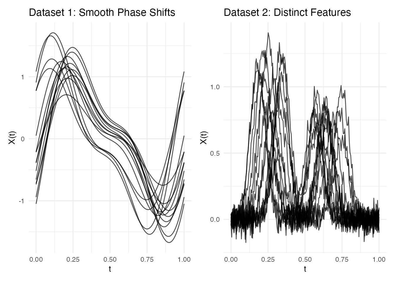

Method 1: Elastic Alignment

Elastic alignment finds the globally optimal warping function by minimizing the $L^2$ distance between SRSFs via dynamic programming. It requires no feature detection and produces smooth, diffeomorphic warping functions.

Mathematical basis: minimize $\|\, q_1 - (q_2 \circ \gamma) \sqrt{\dot\gamma}\,\|_{L^2}^2$ over the warping group $\Gamma$ , where $q_i$ is the SRSF of $f_i$ .

ea_smooth <- elastic.align(fd_smooth)
ea_feat <- elastic.align(fd_feat)

p1 <- plot(ea_smooth, type = "aligned") + labs(title = "Elastic (smooth data)")
p2 <- plot(ea_feat, type = "aligned") + labs(title = "Elastic (feature data)")
p1 + p2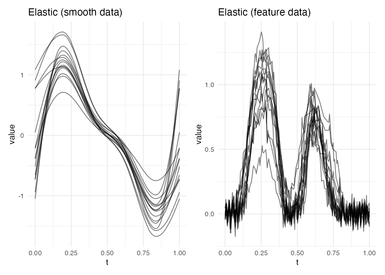

Method 2: Landmark Registration

Landmark registration detects features (peaks, valleys, etc.) and warps curves so that corresponding features align to common target positions. The warping is piecewise-linear between anchor points.

Mathematical basis: For landmarks $\tau_{i,j}$ and targets $\tau_j^*$ , construct $\gamma_i$ as a piecewise-linear function satisfying $\gamma_i(\tau_j^*) = \tau_{i,j}$ .

lr_smooth <- landmark.register(fd_smooth, kind = "peak", min.prominence = 0.3,
                                expected.count = 1)
lr_feat <- landmark.register(fd_feat, kind = "peak", min.prominence = 0.2,
                              expected.count = 2)

p1 <- plot(lr_smooth, type = "registered") +
  labs(title = "Landmark (smooth data)")
p2 <- plot(lr_feat, type = "registered") +
  labs(title = "Landmark (feature data)")
p1 + p2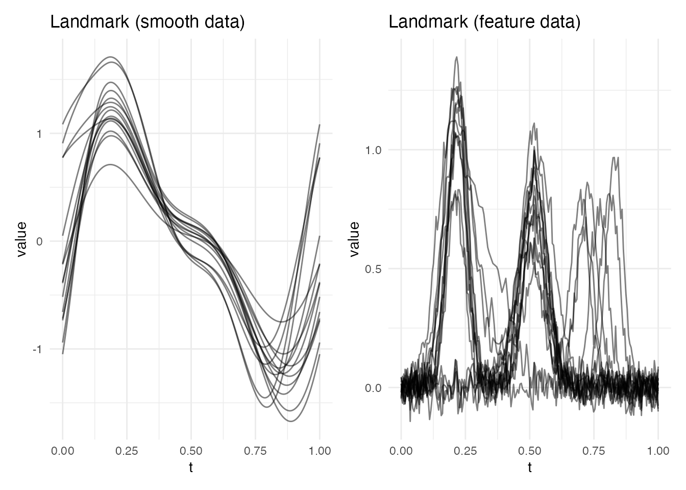

Method 3: Constrained Elastic Alignment

Constrained elastic alignment combines the smooth, globally optimal warping of elastic alignment with landmark pass-through constraints. The warping is computed by segmented dynamic programming between landmark anchor points.

Mathematical basis: minimize $\|q_1 - (q_2 \circ \gamma) \sqrt{\dot\gamma}\|_{L^2}^2$ subject to $\gamma(\tau_j^*) = \tau_{i,j}$ for each landmark pair.

ec_smooth <- elastic.align.constrained(fd_smooth, kind = "peak",
                                        min.prominence = 0.3,
                                        expected.count = 1)
ec_feat <- elastic.align.constrained(fd_feat, kind = "peak",
                                      min.prominence = 0.2,
                                      expected.count = 2)

p1 <- plot(ec_smooth, type = "aligned") +
  labs(title = "Constrained (smooth data)")
p2 <- plot(ec_feat, type = "aligned") +
  labs(title = "Constrained (feature data)")
p1 + p2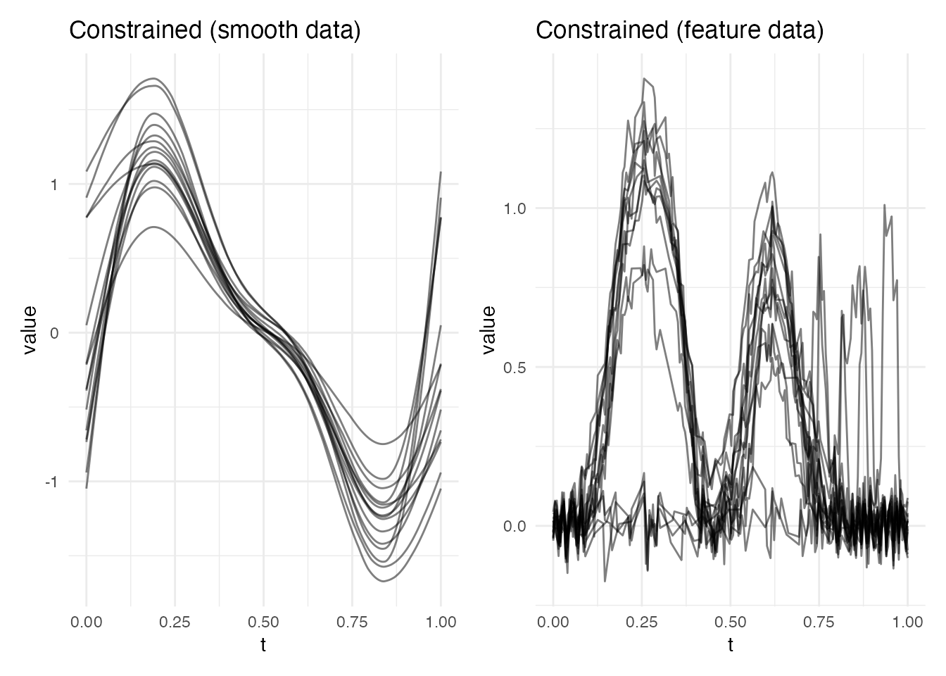

Warping Function Comparison

The warping functions reveal the fundamental difference between methods. Elastic produces smooth warps, landmark produces piecewise-linear warps, and constrained is smooth but passes through landmark anchor points:

p1 <- plot(ea_feat, type = "warps") + labs(title = "Elastic Warps")
p2 <- plot(lr_feat, type = "warps") + labs(title = "Landmark Warps")
p3 <- plot(ec_feat, type = "warps") + labs(title = "Constrained Warps")
p1 + p2 + p3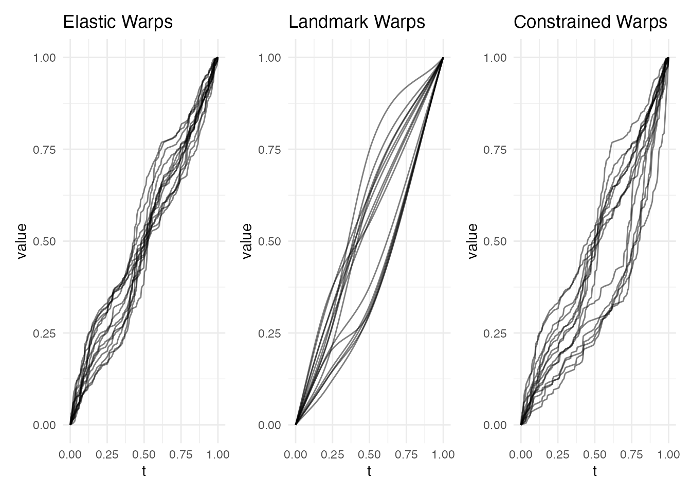

Quantitative Comparison

Variance Reduction

Variance reduction (VR) measures how much pointwise variance is removed by alignment. Higher VR means more phase variability was captured:

$\text{VR} = 1 - \frac{\text{mean pointwise variance (aligned)}}{\text{mean pointwise variance (original)}}$

vr <- function(original, aligned) {
  var_orig <- mean(apply(original$data, 2, var))
  var_aligned <- mean(apply(aligned$data, 2, var))
  1 - var_aligned / var_orig
}

results <- data.frame(
  Dataset = rep(c("Smooth shifts", "Distinct features"), each = 3),
  Method = rep(c("Elastic", "Landmark", "Constrained"), 2),
  VR = c(
    vr(fd_smooth, ea_smooth$aligned),
    vr(fd_smooth, lr_smooth$registered),
    vr(fd_smooth, ec_smooth$aligned),
    vr(fd_feat, ea_feat$aligned),
    vr(fd_feat, lr_feat$registered),
    vr(fd_feat, ec_feat$aligned)
  )
)

results$VR <- round(results$VR, 3)
print(results)
#>             Dataset      Method    VR
#> 1     Smooth shifts     Elastic 0.527
#> 2     Smooth shifts    Landmark 0.380
#> 3     Smooth shifts Constrained 0.527
#> 4 Distinct features     Elastic 0.718
#> 5 Distinct features    Landmark 0.248
#> 6 Distinct features Constrained 0.054

ggplot(results, aes(x = Method, y = VR, fill = Dataset)) +
  geom_col(position = "dodge") +
  labs(title = "Variance Reduction by Method",
       y = "Variance Reduction (higher = better)") +
  scale_fill_manual(values = c("Smooth shifts" = "steelblue",
                                "Distinct features" = "coral")) +
  ylim(0, 1)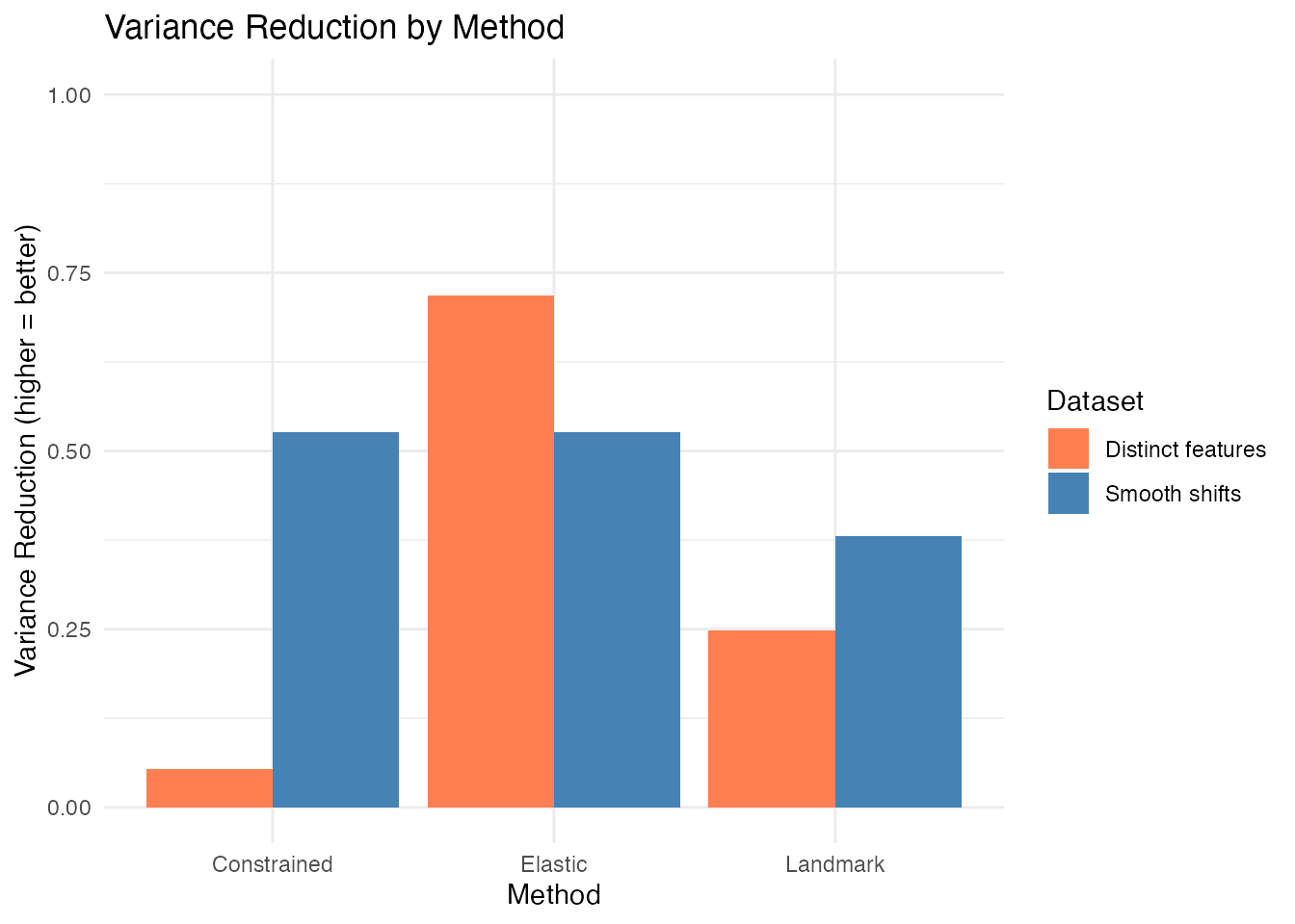

Alignment Quality Diagnostics

For the Karcher mean (elastic), we can compute detailed diagnostics:

km_smooth <- karcher.mean(fd_smooth, max.iter = 15)
aq_smooth <- alignment.quality(fd_smooth, km_smooth)
print(aq_smooth)
#> Alignment Quality Diagnostics
#>   Mean warp complexity: 0.1574 
#>   Mean warp smoothness: 94.7516 
#>   Total variance:      0.1426 
#>   Amplitude variance:  0.0668 
#>   Phase variance:      0.0758 
#>   Phase/Total ratio:   0.5316 
#>   Mean VR:             0.4576

Amplitude-Phase Decomposition

Elastic alignment uniquely provides a principled decomposition of total variability into amplitude and phase components:

plot(aq_smooth, type = "variance")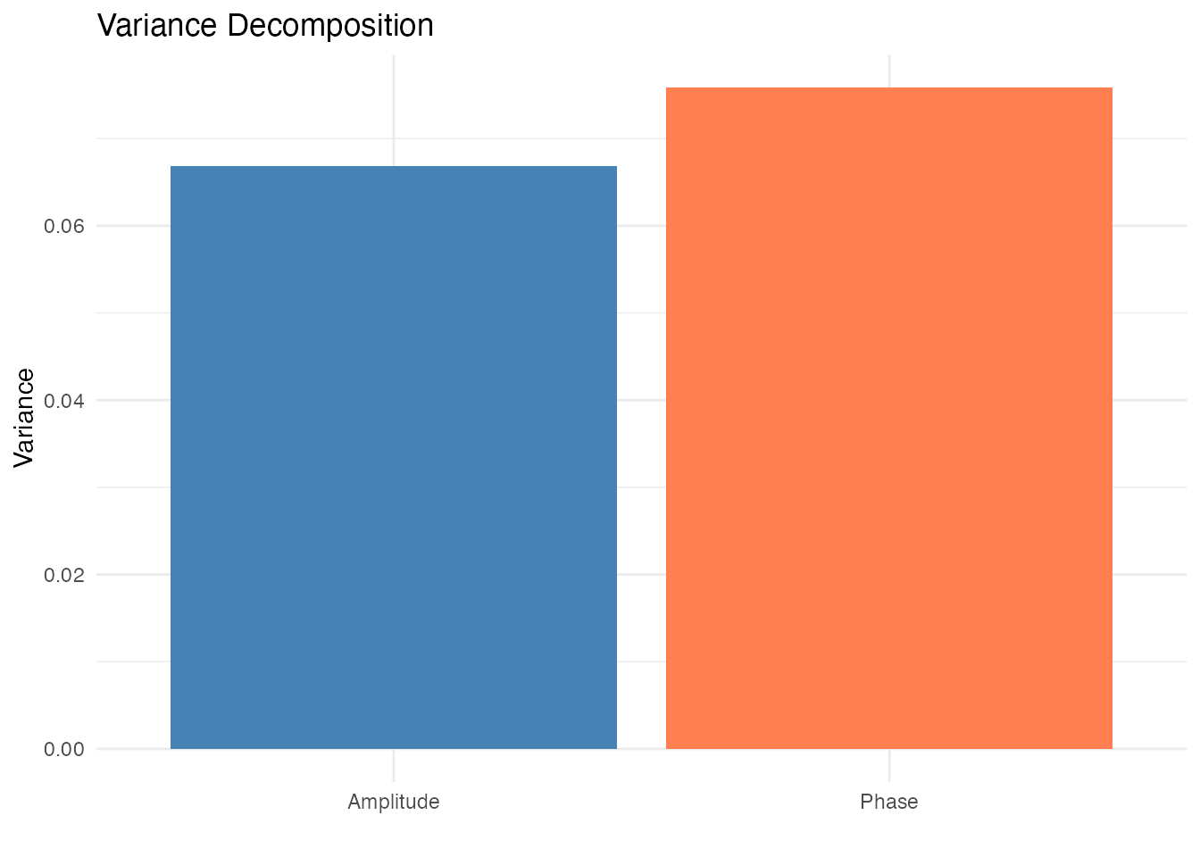

When Methods Succeed and Fail

The examples above use well-behaved data. Real data is messier. This section shows targeted scenarios where each method shines and where it breaks down, so you can match the method to your data.

Scenario 1: Elastic Excels — Smooth Global Warping

When curves differ only by smooth, continuous timing changes with no distinct features, elastic alignment is ideal. It finds the optimal warping without needing any manual tuning:

set.seed(101)
argvals <- seq(0, 1, length.out = 200)
n <- 12

# Smooth curves with continuous phase variation
data_global <- matrix(0, n, 200)
for (i in 1:n) {
  # Smooth nonlinear warp of the time axis
  warp_strength <- runif(1, -0.15, 0.15)
  t_warped <- argvals + warp_strength * sin(pi * argvals)
  t_warped <- (t_warped - min(t_warped)) / (max(t_warped) - min(t_warped))
  amp <- rnorm(1, 1, 0.1)
  data_global[i, ] <- amp * (sin(2 * pi * t_warped) + 0.3 * cos(6 * pi * t_warped))
}
fd_global <- fdata(data_global, argvals = argvals)

ea_global <- elastic.align(fd_global)

# Landmark registration struggles: no clear isolated peaks
lr_global <- tryCatch(
  landmark.register(fd_global, kind = "peak", min.prominence = 0.3, expected.count = 1),
  error = function(e) NULL
)

p1 <- plot(fd_global) + labs(title = "Original: Smooth Warping")
p2 <- plot(ea_global, type = "aligned") + labs(title = "Elastic: Clean alignment")
if (!is.null(lr_global)) {
  p3 <- plot(lr_global, type = "registered") + labs(title = "Landmark: Misses subtlety")
  p1 + p2 + p3 + plot_layout(ncol = 3)
} else {
  p3 <- ggplot() + annotate("text", x = 0.5, y = 0.5,
    label = "Landmark failed:\nno consistent features found",
    size = 4, hjust = 0.5) + theme_void() + labs(title = "Landmark: Failed")
  p1 + p2 + p3 + plot_layout(ncol = 3)
}

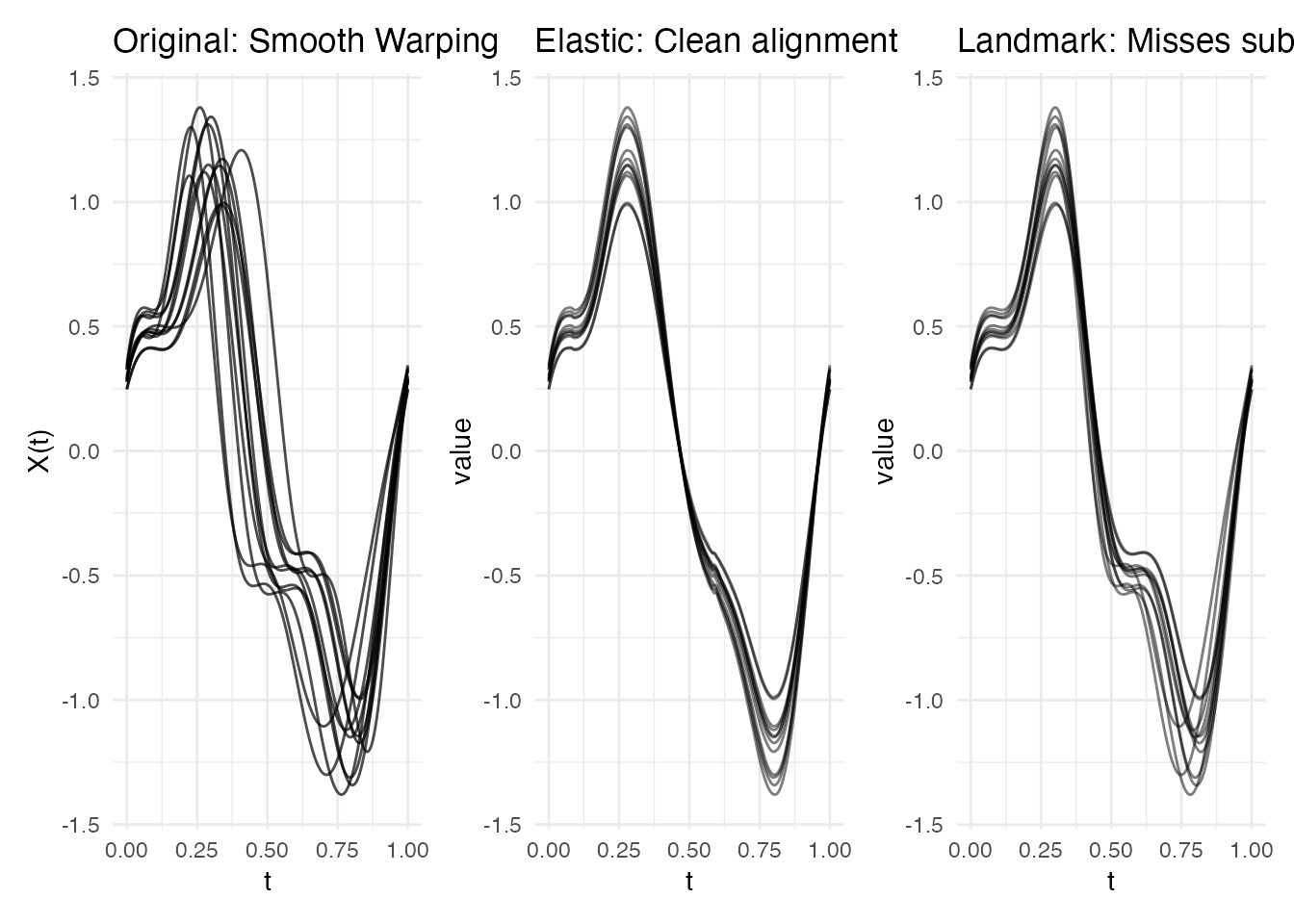
Why elastic wins: The Fisher-Rao metric captures continuous phase variation naturally. Landmark registration needs identifiable features, and these smooth curves have overlapping, broad oscillations with no clear anchor points.

Scenario 2: Landmark Excels — Identifiable Features Shifting Independently

When curves have clearly defined peaks or valleys that shift to different positions, landmark registration directly targets what matters:

# Two-peak curves where peaks shift independently
data_peaks <- matrix(0, n, 200)
for (i in 1:n) {
  pk1_pos <- runif(1, 0.15, 0.35)
  pk2_pos <- runif(1, 0.6, 0.8)
  h1 <- rnorm(1, 1.5, 0.2)
  h2 <- rnorm(1, 1.0, 0.15)
  data_peaks[i, ] <- h1 * exp(-300 * (argvals - pk1_pos)^2) +
                      h2 * exp(-300 * (argvals - pk2_pos)^2)
}
fd_peaks <- fdata(data_peaks, argvals = argvals)

lr_peaks <- landmark.register(fd_peaks, kind = "peak", min.prominence = 0.3,
                               expected.count = 2)
ea_peaks <- elastic.align(fd_peaks)

p1 <- plot(fd_peaks) + labs(title = "Original: Two Shifting Peaks")
p2 <- plot(lr_peaks, type = "registered") + labs(title = "Landmark: Peaks aligned")
p3 <- plot(ea_peaks, type = "aligned") + labs(title = "Elastic: May swap features")
p1 + p2 + p3 + plot_layout(ncol = 3)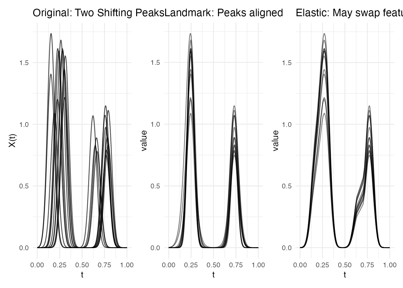

Why landmark wins: It guarantees that peak 1 aligns to peak 1 and peak 2 to peak 2. Elastic alignment has no feature awareness — it minimizes overall distance, which can sometimes swap or merge features when they are far apart.

Scenario 3: Elastic Struggles — Noisy Data

When curves are noisy, elastic alignment’s dynamic programming can over-warp, matching noise spikes rather than underlying signal. The solution: smooth first, then align:

# Clean signal + heavy noise
data_noisy <- matrix(0, n, 200)
for (i in 1:n) {
  shift <- runif(1, -0.08, 0.08)
  signal <- sin(2 * pi * (argvals - shift))
  data_noisy[i, ] <- signal + rnorm(200, 0, 0.4)
}
fd_noisy <- fdata(data_noisy, argvals = argvals)

# Direct alignment on noisy data: over-warping
ea_noisy_raw <- elastic.align(fd_noisy)

# Better approach: smooth first, then align
fd_smooth_noisy <- fdata(t(apply(fd_noisy$data, 1, function(y) {
  stats::smooth.spline(argvals, y, spar = 0.6)$y
})), argvals = argvals)
ea_noisy_smooth <- elastic.align(fd_smooth_noisy)

p1 <- plot(fd_noisy) + labs(title = "Original: Noisy Curves")
p2 <- plot(ea_noisy_raw, type = "aligned") +
  labs(title = "Elastic on raw: Over-warps")
p3 <- plot(ea_noisy_smooth, type = "aligned") +
  labs(title = "Smooth then align: Controlled")
p1 + p2 + p3 + plot_layout(ncol = 3)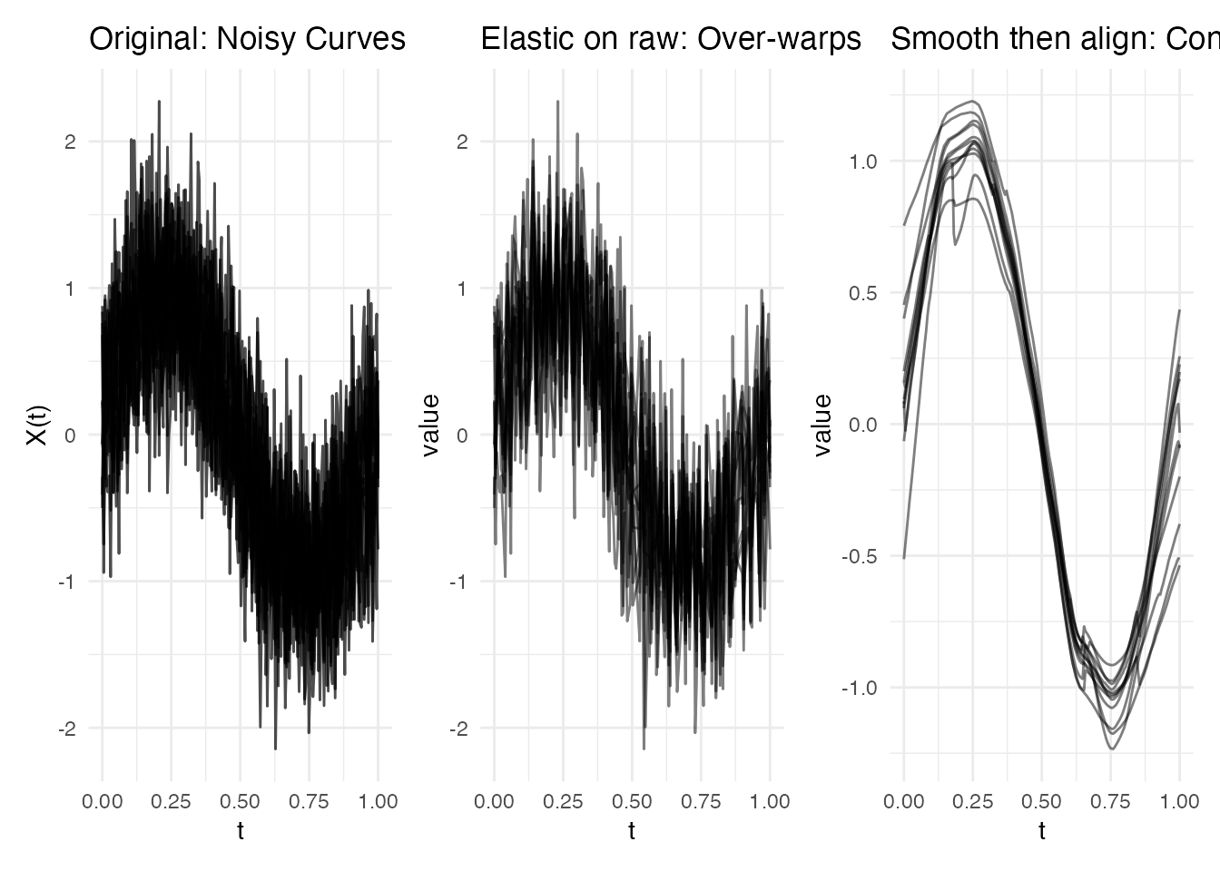

p4 <- plot(ea_noisy_raw, type = "warps") +
  labs(title = "Warps (raw): Overly complex")
p5 <- plot(ea_noisy_smooth, type = "warps") +
  labs(title = "Warps (smoothed): Reasonable")
p4 + p5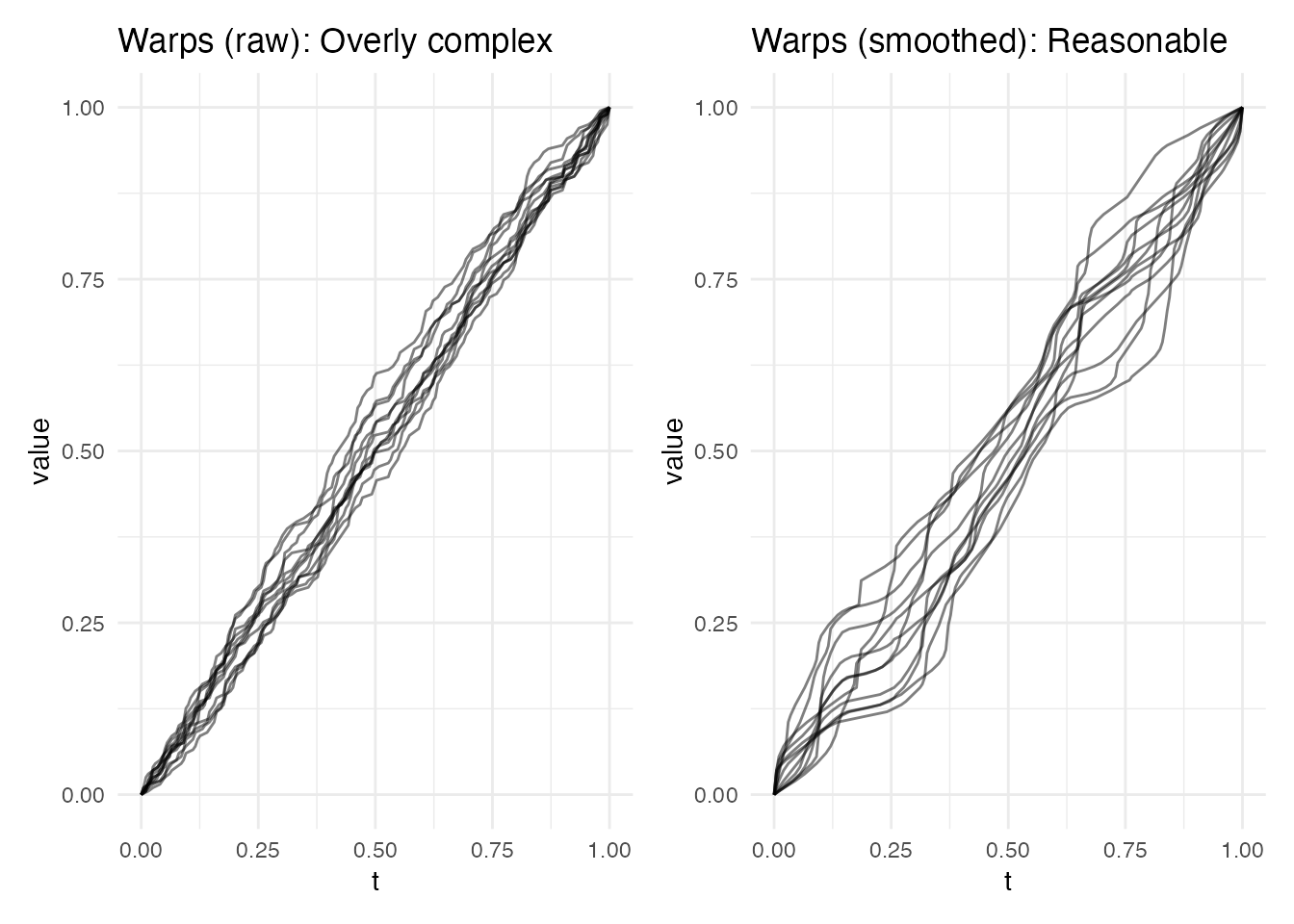

Lesson: Always smooth noisy data before elastic alignment. The SRSF transform amplifies noise (it involves a derivative), causing the dynamic programming to match noise spikes. Pre-smoothing with splines or a kernel smoother prevents over-warping. Alternatively, use karcher.mean() with its lambda parameter to penalize warp complexity.

Scenario 4: Landmark Struggles — Variable Number of Features

When curves have different numbers of features, landmark registration with a fixed expected.count forces all curves into the same template. This can produce artifacts:

data_var <- matrix(0, n, 200)
for (i in 1:n) {
  # Some curves have 1 peak, others have 2
  if (i <= n/2) {
    pk1 <- runif(1, 0.3, 0.5)
    data_var[i, ] <- 1.5 * exp(-300 * (argvals - pk1)^2)
  } else {
    pk1 <- runif(1, 0.2, 0.35)
    pk2 <- runif(1, 0.6, 0.75)
    data_var[i, ] <- exp(-300 * (argvals - pk1)^2) + exp(-300 * (argvals - pk2)^2)
  }
  data_var[i, ] <- data_var[i, ] + 0.02 * rnorm(200)
}
fd_var <- fdata(data_var, argvals = argvals)

# Landmark fails gracefully but results are unreliable
lr_var <- tryCatch(
  landmark.register(fd_var, kind = "peak", min.prominence = 0.2, expected.count = 2),
  error = function(e) NULL
)
ea_var <- elastic.align(fd_var)

p1 <- plot(fd_var) + labs(title = "Original: Mixed 1-peak & 2-peak")
p2 <- plot(ea_var, type = "aligned") + labs(title = "Elastic: Handles gracefully")
if (!is.null(lr_var)) {
  p3 <- plot(lr_var, type = "registered") +
    labs(title = "Landmark: Forced 2-peak template")
} else {
  p3 <- ggplot() + annotate("text", x = 0.5, y = 0.5,
    label = "Landmark failed:\ncannot find 2 peaks in all curves",
    size = 4, hjust = 0.5) + theme_void() + labs(title = "Landmark: Failed")
}
p1 + p2 + p3 + plot_layout(ncol = 3)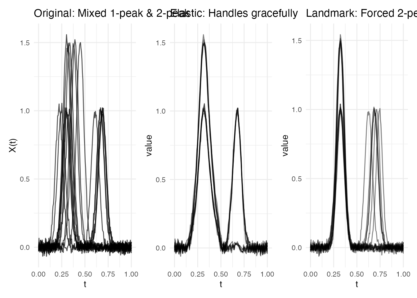

Why elastic wins here: It makes no assumptions about features. When curves have genuinely different shapes, elastic alignment finds the best continuous warping for each pair. Landmark registration requires a consistent feature template across all curves.

Scenario 5: Constrained Excels — Best of Both Worlds

When you have identifiable features AND want smooth warping between them, constrained elastic alignment is the best choice:

# ECG-like data: sharp features + smooth variation between them
data_ecg <- matrix(0, n, 200)
for (i in 1:n) {
  r_pos <- runif(1, 0.3, 0.45)
  t_pos <- runif(1, 0.55, 0.7)
  # R-wave (tall sharp peak)
  r_wave <- 2.0 * exp(-800 * (argvals - r_pos)^2)
  # T-wave (broader, shorter)
  t_wave <- 0.6 * exp(-100 * (argvals - t_pos)^2)
  # Baseline wander
  baseline <- 0.15 * sin(2 * pi * argvals + runif(1, 0, 2*pi))
  data_ecg[i, ] <- r_wave + t_wave + baseline + 0.03 * rnorm(200)
}
fd_ecg <- fdata(data_ecg, argvals = argvals)

ea_ecg <- elastic.align(fd_ecg)
lr_ecg <- landmark.register(fd_ecg, kind = "peak", min.prominence = 0.3,
                             expected.count = 2)
ec_ecg <- elastic.align.constrained(fd_ecg, kind = "peak",
                                     min.prominence = 0.3,
                                     expected.count = 2)

p1 <- plot(fd_ecg) + labs(title = "Original: ECG-like")
p2 <- plot(ea_ecg, type = "aligned") + labs(title = "Elastic: Good overall")
p3 <- plot(lr_ecg, type = "registered") +
  labs(title = "Landmark: Peaks aligned, warps angular")
p4 <- plot(ec_ecg, type = "aligned") +
  labs(title = "Constrained: Peaks aligned + smooth warps")
(p1 + p2) / (p3 + p4)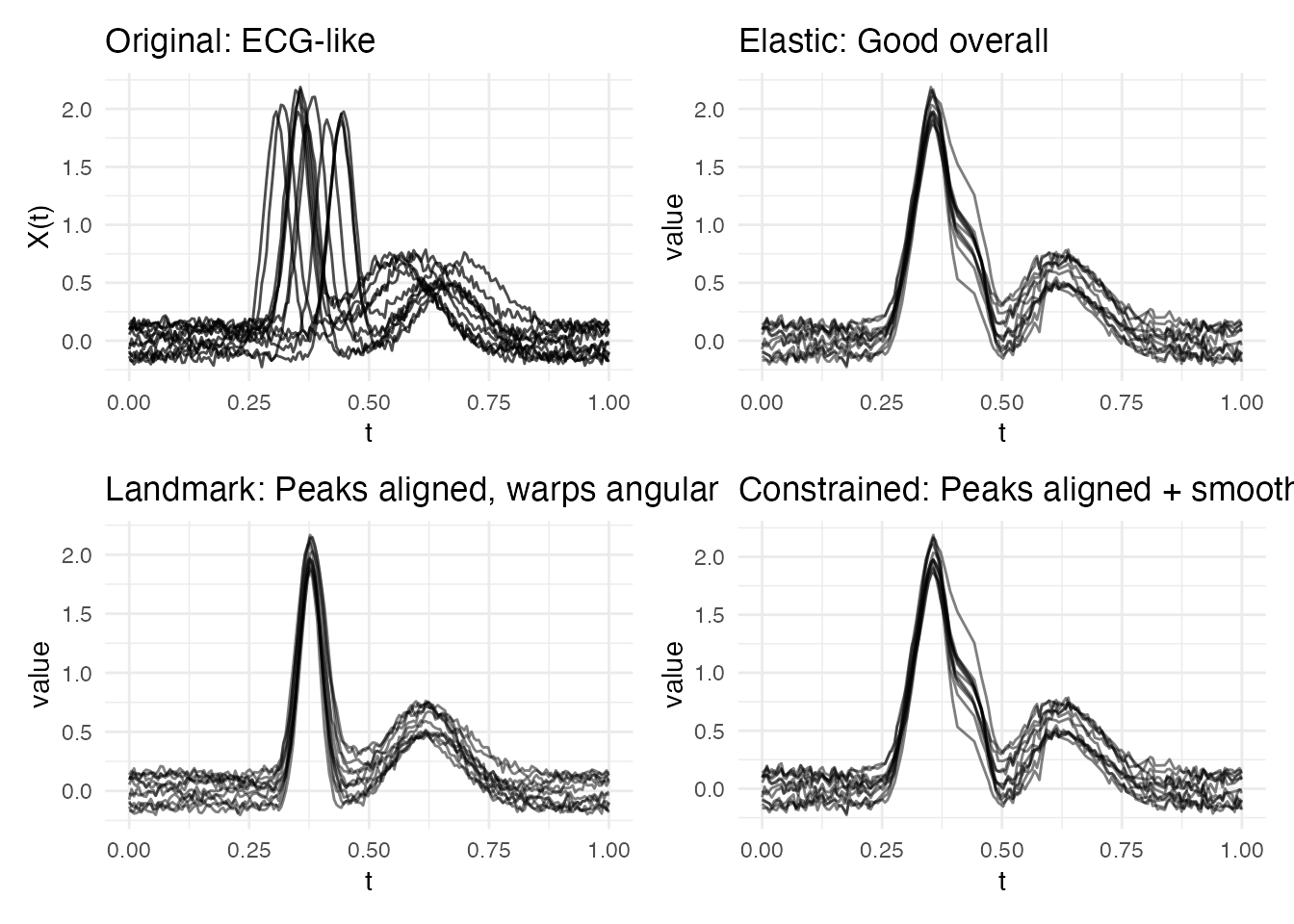

p5 <- plot(ea_ecg, type = "warps") + labs(title = "Elastic warps")
p6 <- plot(lr_ecg, type = "warps") + labs(title = "Landmark warps (piecewise-linear)")
p7 <- plot(ec_ecg, type = "warps") + labs(title = "Constrained warps (smooth + anchored)")
p5 + p6 + p7 + plot_layout(ncol = 3)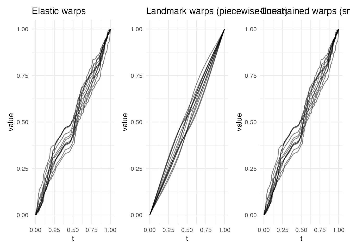

Why constrained wins: The R-wave and T-wave are clinically meaningful features that must correspond correctly (landmark guarantee). But between these features, elastic optimization produces smoother warps than the piecewise-linear interpolation of pure landmark registration.

Scenario Summary

Scenario	Best method	Why
Smooth global warping	Elastic	No features to anchor; elastic finds optimal continuous warp
Independent feature shifts	Landmark	Guarantees feature correspondence
Noisy data	Elastic (with lambda)	Lambda penalty controls over-warping
Variable number of features	Elastic	No feature template required
Features + smooth variation	Constrained	Combines feature anchoring with smooth optimization

Decision Guide

Summary Table

Method	Warping	Automation	Speed	Smoothness	Feature control
Elastic	Smooth diffeomorphism	Fully automatic	$O(nm^2)$	High	None
Landmark	Piecewise-linear	Needs feature type	$O(nm + nk)$	Low (corners at landmarks)	Full
Constrained	Smooth with anchors	Needs feature type	$O(nm^2/k)$	High (between landmarks)	Partial
TSRVF	(uses elastic)	Fully automatic	$O(nm^2)$ + PCA	High	None

When to Use Each Method

Use elastic alignment when:

You have no prior knowledge about which features should correspond
Curves have smooth, continuous timing differences
You want a principled metric space structure (Fisher-Rao distance)
You need amplitude-phase decomposition or TSRVF for downstream analysis

Use landmark registration when:

Features are well-defined and domain-meaningful (ECG waves, spectral peaks)
You need guaranteed feature correspondence
Speed is critical (linear in grid size per landmark)
Curves have complex warping that confuses global DP (e.g., features moving in opposite directions)

Use constrained elastic alignment when:

You want both smooth warps and feature correspondence
Some features must align exactly, but the warping between them should be optimized
You are comparing elastic and landmark results and want a middle ground

Use TSRVF when:

You need to perform PCA, regression, or classification on aligned data
You want a Euclidean representation of curve shapes
You have already computed a Karcher mean and want to extract tangent vectors

Pitfalls

Method	Common pitfall	Mitigation
Elastic	Over-warping (pinching) on noisy data	Increase `lambda` penalty
Landmark	Mismatched landmark correspondence	Use `expected.count`, increase `min.prominence`
Constrained	Too few landmarks = barely constrained	Detect multiple landmark types
TSRVF	Linearization error for curves far from mean	Check reconstruction quality

Workflow Example

A typical analysis workflow combining multiple methods:

# 1. Explore data
plot(fd_feat) + labs(title = "Step 1: Explore")

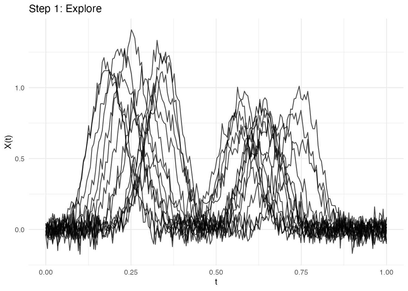
# 2. Detect features to understand structure
lms <- detect.landmarks(fd_feat, kind = "peak", min.prominence = 0.2)
cat("Landmarks per curve:",
    paste(sapply(lms, nrow), collapse = ", "), "\n")
#> Landmarks per curve: 3, 2, 3, 5, 2, 2, 3, 2, 4, 2, 4, 2, 2, 3, 3

# 3. Align (choose method based on data)
lr <- landmark.register(fd_feat, kind = "peak", min.prominence = 0.2,
                         expected.count = 2)

# 4. For downstream analysis, compute Karcher mean + TSRVF
km <- karcher.mean(lr$registered, max.iter = 10)
tv <- tsrvf.from.alignment(km)

# 5. Standard PCA on tangent vectors
pca <- prcomp(tv$tangent_vectors$data)
var_exp <- cumsum(pca$sdev^2 / sum(pca$sdev^2))
cat("Variance explained (first 3 PCs):",
    round(var_exp[1:3] * 100, 1), "%\n")
#> Variance explained (first 3 PCs): 16.5 28.8 39.9 %