Elastic Changepoint Detection

Overview

Changepoint detection identifies the index at which a chronologically ordered sequence of functional observations undergoes a structural change. The elastic.changepoint() function provides three approaches, each sensitive to a different type of change:

• Amplitude changepoints: Detect shifts in functional shape
• Phase changepoints: Detect shifts in feature timing
• FPCA changepoints: Detect changes in principal component structure (sensitive to both amplitude and phase)

Two Time Indices

Functional changepoint detection involves two distinct time axes:

• Intra-curve time $t \in \mathcal{T}$: the domain over which each individual curve is observed (the argvals of the fdata object). For example, $t$ might represent seconds within a single production cycle or hours within a single day.
• Inter-curve index $i = 1,\ldots,n$: the chronological ordering of curves (the row index in the fdata object). For example, $i$ might index successive production runs, calendar days, or patient visits.

The changepoint $\tau$ is detected on the inter-curve axis: “at which curve index does the distribution of curves change?” The intra-curve domain $t$ is used internally to compute distances, align SRVFs, and extract FPCA features.

Important: The rows of the fdata object must be in chronological order. Shuffling the rows would destroy the sequential structure that the CUSUM test relies on.

Mathematical Framework

CUSUM Test for Functional Data

Given a functional time series $\{f_1,\ldots,f_n\}$ ordered chronologically by the inter-curve index $i$, we test $H_0$: no changepoint (the distribution is stationary across $i$) against $H_1$: there exists $\tau \in \{1,\ldots,n-1\}$ such that the distribution changes at $\tau$.

The CUSUM (cumulative sum) statistic for a scalar summary $S_i$ extracted from each curve is

$$T_n(k) = \frac{1}{\hat{\sigma}\sqrt{n}} \left| \sum_{i=1}^{k} S_i - \frac{k}{n}\sum_{i=1}^{n} S_i \right|, \qquad k = 1,\ldots,n-1,$$

and the test statistic is $T_n = \max_{k} T_n(k)$, with the estimated changepoint $\hat{\tau} = \arg\max_{k} T_n(k)$.

How the Summary Statistic Differs

• Amplitude: $S_i^{(\text{amp})} = \|\tilde{q}_i - \bar{q}\|_2$ (distance between aligned SRVF and Karcher mean SRVF). Sensitive to shape changes only.
• Phase: $S_i^{(\text{ph})} = d_{\Gamma}(\gamma_i, \text{id})$ (elastic distance between warp function and the identity). Sensitive to timing changes only.
• FPCA: Multivariate CUSUM on the FPC scores $\boldsymbol{\xi}_i$. Sensitive to changes in either amplitude, phase, or both.

Permutation Inference

Under $H_0$, the ordering of curves is exchangeable. The p-value is estimated by randomly permuting the sequence $B$ times:

$$\hat{p} = \frac{1}{B}\sum_{b=1}^{B} \mathbf{1}\{T_n^{(b)} \geq T_n\}.$$

Example 1: Pure Amplitude Changepoint

In this scenario, the shape of the curves changes at $\tau = 30$ but the timing stays the same. Before the break: simple sine waves. After: the amplitude doubles and a second harmonic appears.

curves_amp <- matrix(0, n, m)
for (i in 1:tau)
  curves_amp[i, ] <- sin(2 * pi * t) + rnorm(m, sd = 0.12)
for (i in (tau + 1):n)
  curves_amp[i, ] <- 2 * sin(2 * pi * t) + 0.8 * sin(4 * pi * t) +
                     rnorm(m, sd = 0.12)
fd_amp <- fdata(curves_amp, argvals = t)

plot(fd_amp, main = "Example 1: Pure Amplitude Change at obs 30",
     xlab = "t", ylab = "X(t)")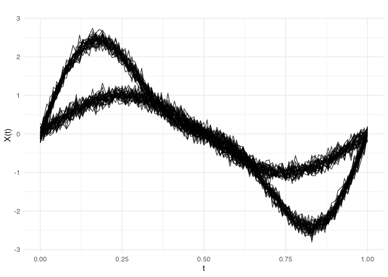

We run both the amplitude and phase tests. Since only shape changed, the amplitude test should produce a much larger CUSUM statistic:

res_amp_a <- elastic.changepoint(fd_amp, type = "amplitude", n.mc = 199, seed = 42)
res_amp_p <- elastic.changepoint(fd_amp, type = "phase", n.mc = 199, seed = 42)

cat("Amplitude test: detected at", res_amp_a$changepoint,
    "| CUSUM =", round(res_amp_a$test.statistic, 5),
    "| p =", format(res_amp_a$p.value, digits = 3), "\n")
#> Amplitude test: detected at 30 | CUSUM = 0.05105 | p = 0.005
cat("Phase test:     detected at", res_amp_p$changepoint,
    "| CUSUM =", round(res_amp_p$test.statistic, 5),
    "| p =", format(res_amp_p$p.value, digits = 3), "\n")
#> Phase test:     detected at 30 | CUSUM = 0.00255 | p = 0.005
cat("Amplitude/Phase CUSUM ratio:", round(res_amp_a$test.statistic /
                                     res_amp_p$test.statistic, 1), "x\n")
#> Amplitude/Phase CUSUM ratio: 20 x

The amplitude test is highly significant (small p-value) with a much larger CUSUM, confirming the change is in shape, not timing. The phase test may also reach significance because shape changes can induce spurious phase variation, but the CUSUM ratio clearly indicates a shape-driven change.

plot(res_amp_a, type = "statistic")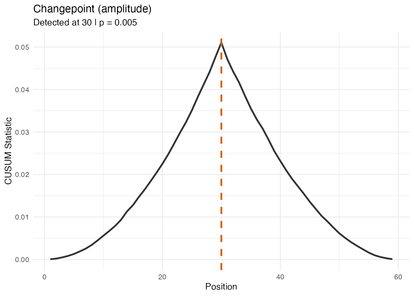

plot(res_amp_a, type = "data")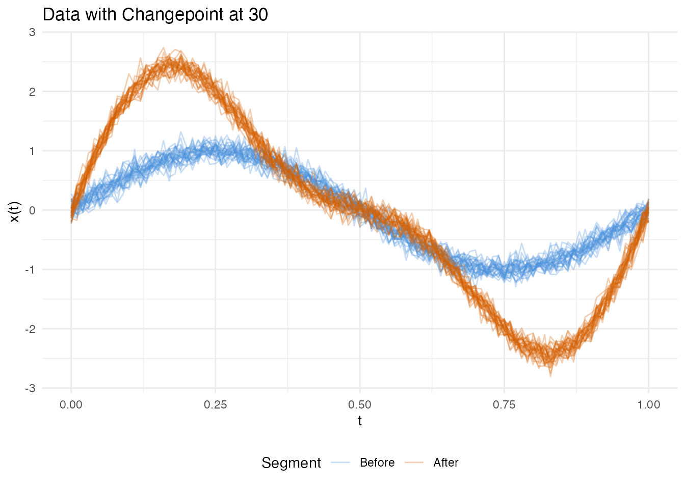

Example 2: Pure Phase Changepoint

Here the shape is identical before and after, but the timing shifts: after $\tau = 30$, the same template is observed through a nonlinear time warp (as if the process runs faster at the start and slower at the end).

template_ph <- sin(2 * pi * t) + 0.4 * cos(4 * pi * t)

curves_ph <- matrix(0, n, m)
for (i in 1:tau)
  curves_ph[i, ] <- template_ph + rnorm(m, sd = 0.12)
for (i in (tau + 1):n) {
  gamma <- pbeta(t, 1.6, 0.7)  # nonlinear warp
  curves_ph[i, ] <- approx(t, template_ph, xout = gamma, rule = 2)$y +
                    rnorm(m, sd = 0.12)
}
fd_ph <- fdata(curves_ph, argvals = t)

plot(fd_ph, main = "Example 2: Pure Phase Change at obs 30",
     xlab = "t", ylab = "X(t)")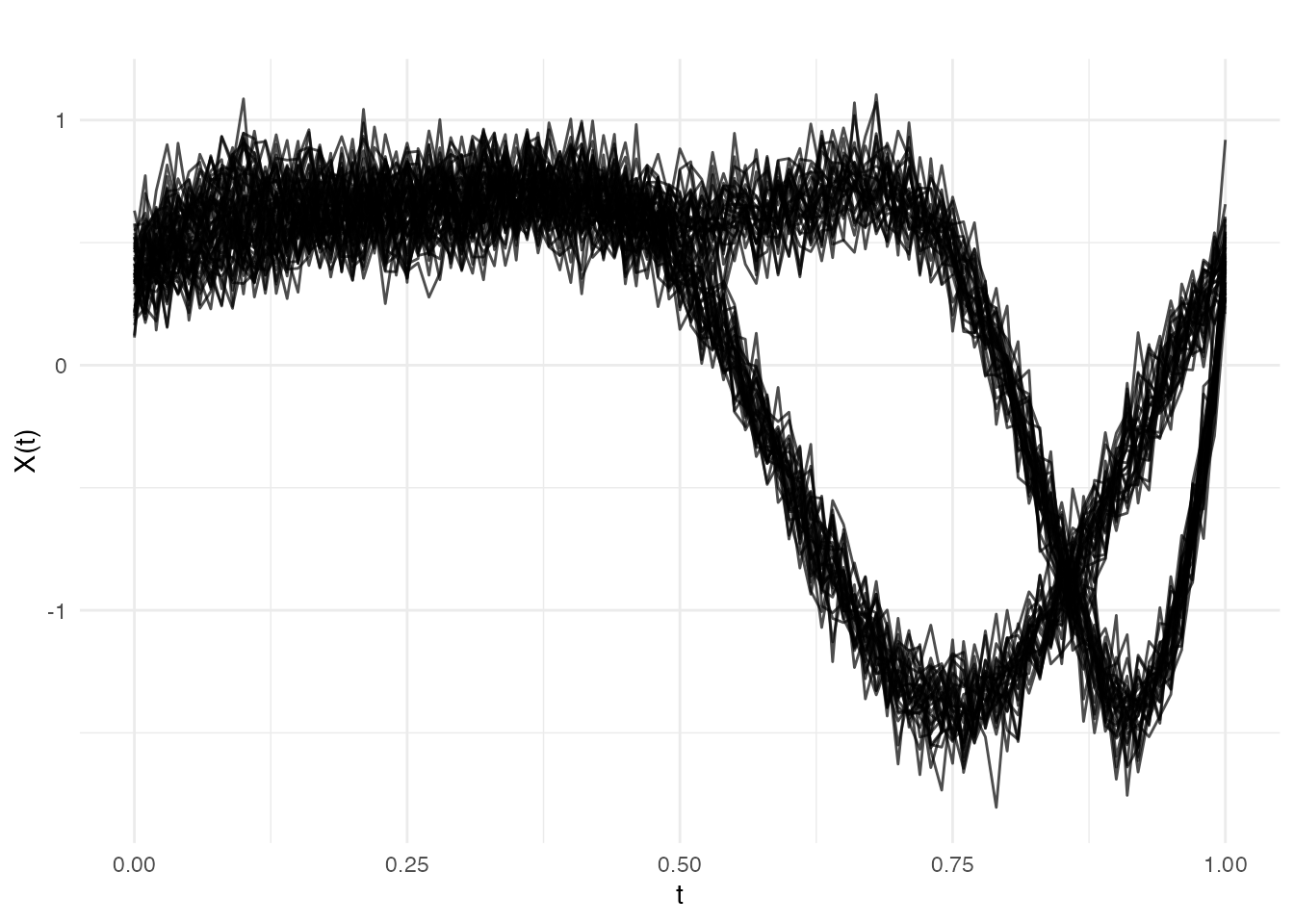

Now the phase test should dominate:

res_ph_a <- elastic.changepoint(fd_ph, type = "amplitude", n.mc = 199, seed = 42)
res_ph_p <- elastic.changepoint(fd_ph, type = "phase", n.mc = 199, seed = 42)

cat("Amplitude test: detected at", res_ph_a$changepoint,
    "| CUSUM =", round(res_ph_a$test.statistic, 5),
    "| p =", format(res_ph_a$p.value, digits = 3), "\n")
#> Amplitude test: detected at 30 | CUSUM = 0.002 | p = 0.005
cat("Phase test:     detected at", res_ph_p$changepoint,
    "| CUSUM =", round(res_ph_p$test.statistic, 5),
    "| p =", format(res_ph_p$p.value, digits = 3), "\n")
#> Phase test:     detected at 30 | CUSUM = 0.00422 | p = 0.005
cat("Phase/Amplitude CUSUM ratio:", round(res_ph_p$test.statistic /
                                     res_ph_a$test.statistic, 1), "x\n")
#> Phase/Amplitude CUSUM ratio: 2.1 x

The phase CUSUM is larger and significant, confirming the change is in timing, not shape.

plot(res_ph_p, type = "statistic")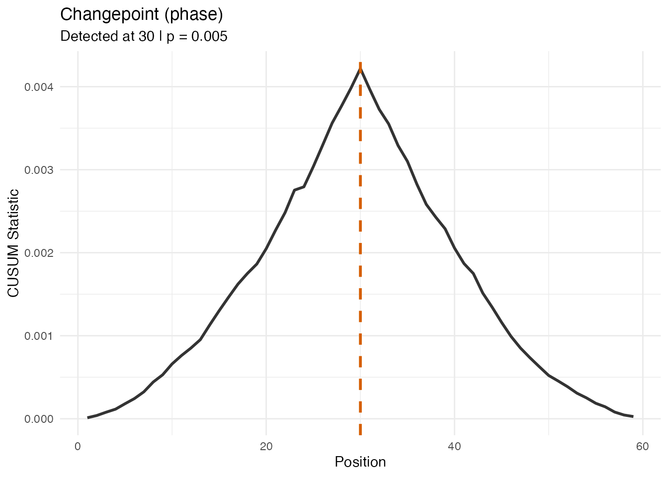

plot(res_ph_p, type = "data")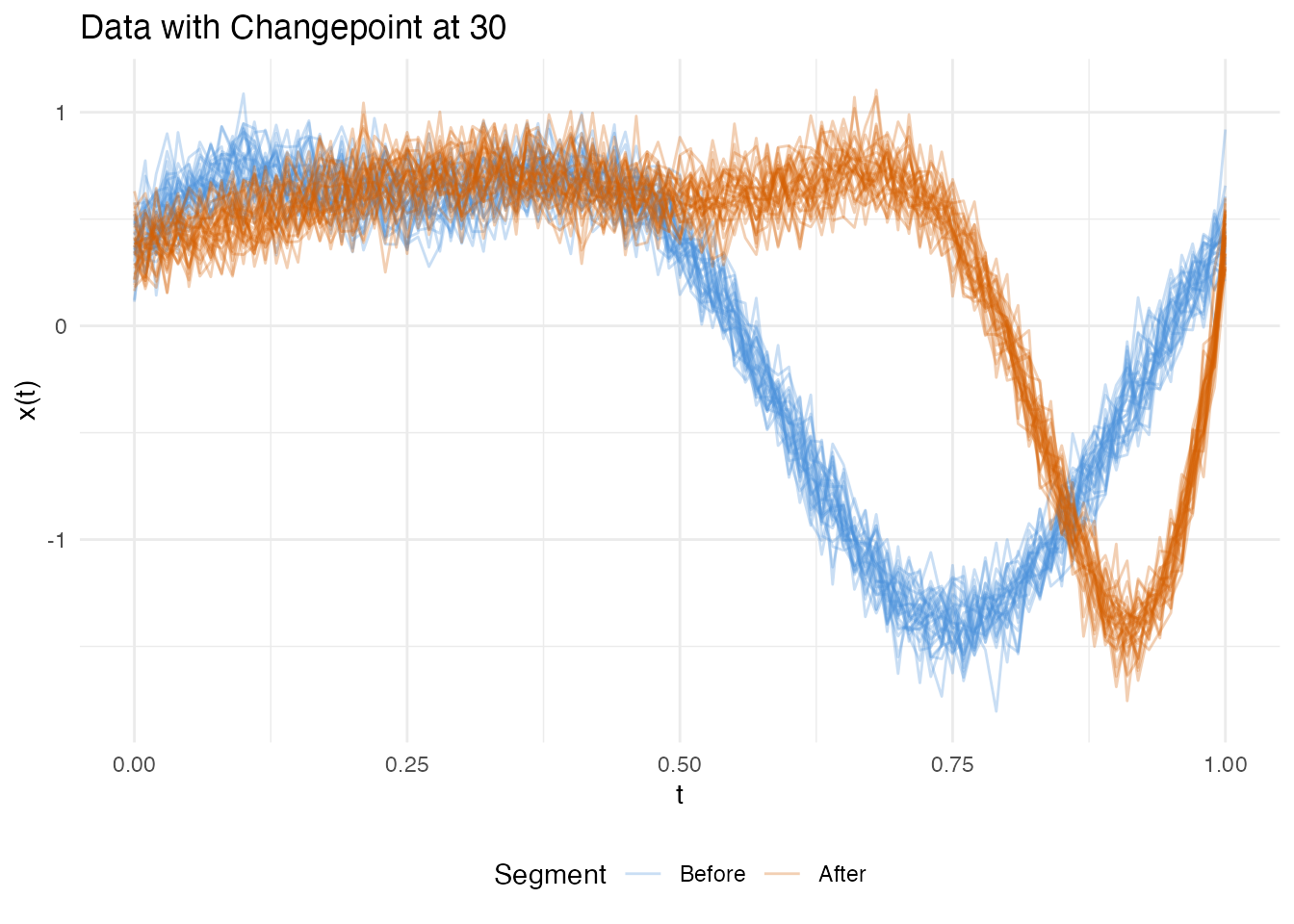

Example 3: Mixed Changepoint (Amplitude + Phase)

In practice, structural breaks often involve both shape and timing changes simultaneously. After $\tau = 30$, the curves are scaled, gain a harmonic, and are nonlinearly warped.

curves_mix <- matrix(0, n, m)
for (i in 1:tau)
  curves_mix[i, ] <- sin(2 * pi * t) + rnorm(m, sd = 0.12)
for (i in (tau + 1):n) {
  gamma <- pbeta(t, 1.4, 0.7)
  template_mix <- 1.5 * sin(2 * pi * t) + 0.5 * cos(4 * pi * t)
  curves_mix[i, ] <- approx(t, template_mix, xout = gamma, rule = 2)$y +
                     rnorm(m, sd = 0.12)
}
fd_mix <- fdata(curves_mix, argvals = t)

plot(fd_mix, main = "Example 3: Mixed Change at obs 30",
     xlab = "t", ylab = "X(t)")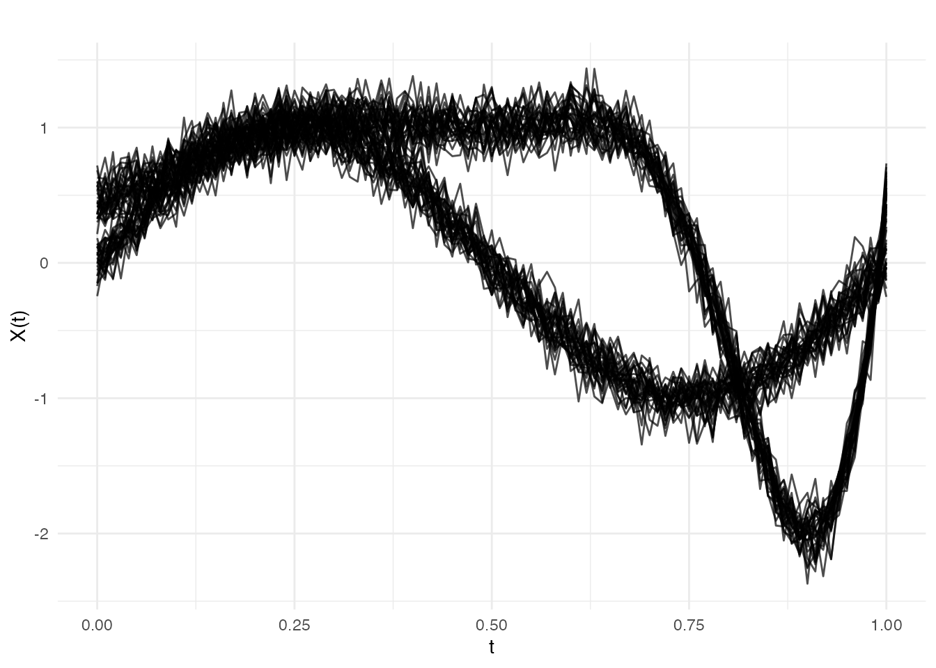

All three tests detect the changepoint, but the FPCA-based test — which captures both amplitude and phase variation — produces the strongest signal:

res_mix_a <- elastic.changepoint(fd_mix, type = "amplitude", n.mc = 199, seed = 42)
res_mix_p <- elastic.changepoint(fd_mix, type = "phase", n.mc = 199, seed = 42)
res_mix_f <- elastic.changepoint(fd_mix, type = "fpca", pca.method = "vertical",
                                 ncomp = 3, n.mc = 199, seed = 42)

cat("Amplitude test: detected at", res_mix_a$changepoint,
    "| CUSUM =", round(res_mix_a$test.statistic, 5),
    "| p =", format(res_mix_a$p.value, digits = 3), "\n")
#> Amplitude test: detected at 30 | CUSUM = 0.02362 | p = 0.005
cat("Phase test:     detected at", res_mix_p$changepoint,
    "| CUSUM =", round(res_mix_p$test.statistic, 5),
    "| p =", format(res_mix_p$p.value, digits = 3), "\n")
#> Phase test:     detected at 30 | CUSUM = 0.00372 | p = 0.005
cat("FPCA test:      detected at", res_mix_f$changepoint,
    "| CUSUM =", round(res_mix_f$test.statistic, 5),
    "| p =", format(res_mix_f$p.value, digits = 3), "\n")
#> FPCA test:      detected at 30 | CUSUM = 0.23432 | p = 0.005

plot(res_mix_f, type = "statistic")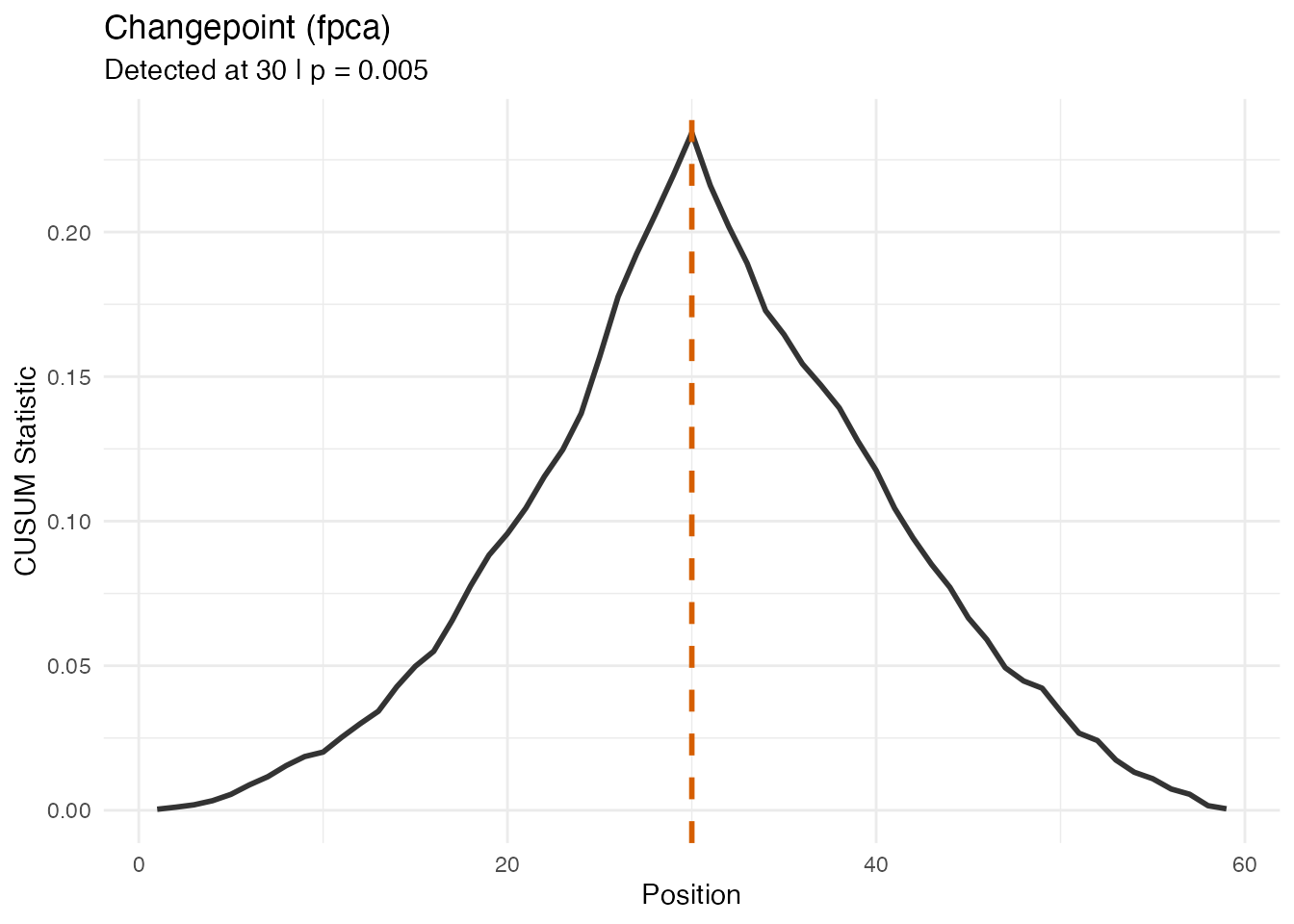

plot(res_mix_f, type = "data")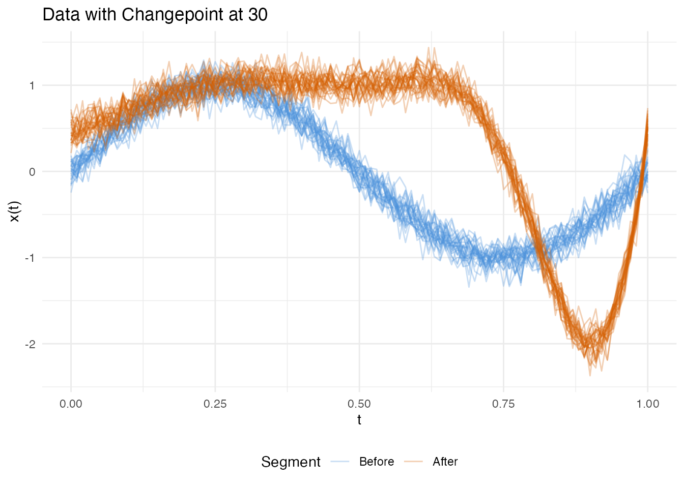

Summary: Which Test for Which Change?

summary_df <- data.frame(
  Example = c("1. Pure Amplitude", "1. Pure Amplitude",
              "2. Pure Phase", "2. Pure Phase",
              "3. Mixed", "3. Mixed", "3. Mixed"),
  Test = c("amplitude", "phase",
           "amplitude", "phase",
           "amplitude", "phase", "fpca"),
  Detected = c(res_amp_a$changepoint, res_amp_p$changepoint,
               res_ph_a$changepoint, res_ph_p$changepoint,
               res_mix_a$changepoint, res_mix_p$changepoint,
               res_mix_f$changepoint),
  CUSUM = round(c(res_amp_a$test.statistic, res_amp_p$test.statistic,
                   res_ph_a$test.statistic, res_ph_p$test.statistic,
                   res_mix_a$test.statistic, res_mix_p$test.statistic,
                   res_mix_f$test.statistic), 5),
  p.value = c(res_amp_a$p.value, res_amp_p$p.value,
              res_ph_a$p.value, res_ph_p$p.value,
              res_mix_a$p.value, res_mix_p$p.value,
              res_mix_f$p.value)
)
knitr::kable(summary_df, digits = c(0, 0, 0, 5, 4))

Example	Test	Detected	CUSUM	p.value
1. Pure Amplitude	amplitude	30	0.05105	0.005
1. Pure Amplitude	phase	30	0.00255	0.005
2. Pure Phase	amplitude	30	0.00200	0.005
2. Pure Phase	phase	30	0.00422	0.005
3. Mixed	amplitude	30	0.02362	0.005
3. Mixed	phase	30	0.00372	0.005
3. Mixed	fpca	30	0.23432	0.005

Change type	Best test	Rationale
Shape only	type = "amplitude"	SRVF distance isolates shape after removing phase
Timing only	type = "phase"	Warp distance isolates timing after alignment
Both	type = "fpca"	FPCA scores capture combined amplitude + phase variation

Quantifying Change Strength

After detecting a changepoint at $\hat{\tau}$, we can quantify how large the change is by comparing the two segments. Two natural effect size measures are:

• L2 effect size: the root-mean-square distance between the mean curves of the before and after segments, $$\Delta_{\text{L2}} = \left(\int_{\mathcal{T}} \bigl(\bar{f}_{\text{before}}(t) - \bar{f}_{\text{after}}(t)\bigr)^2 \, dt\right)^{1/2}.$$
• Relative change: $\Delta_{\text{L2}} / \|\bar{f}_{\text{before}}\|_2 \times 100\%$, expressing the shift as a percentage of the baseline signal magnitude.

effect_size <- function(fdataobj, changepoint) {
  X <- fdataobj$data
  n <- nrow(X)
  before <- colMeans(X[1:changepoint, , drop = FALSE])
  after  <- colMeans(X[(changepoint + 1):n, , drop = FALSE])
  l2 <- sqrt(mean((after - before)^2))
  baseline <- sqrt(mean(before^2))
  list(l2 = l2, relative_pct = l2 / baseline * 100,
       max_pointwise = max(abs(after - before)))
}

# Amplitude example
es_amp <- effect_size(fd_amp, res_amp_a$changepoint)
cat("Example 1 (Amplitude):\n")
#> Example 1 (Amplitude):
cat("  L2 effect size:", round(es_amp$l2, 3), "\n")
#>   L2 effect size: 0.904
cat("  Relative change:", round(es_amp$relative_pct, 1), "%\n")
#>   Relative change: 129.1 %
cat("  Max pointwise diff:", round(es_amp$max_pointwise, 3), "\n\n")
#>   Max pointwise diff: 1.601

# Phase example
es_ph <- effect_size(fd_ph, res_ph_p$changepoint)
cat("Example 2 (Phase):\n")
#> Example 2 (Phase):
cat("  L2 effect size:", round(es_ph$l2, 3), "\n")
#>   L2 effect size: 0.87
cat("  Relative change:", round(es_ph$relative_pct, 1), "%\n")
#>   Relative change: 114.8 %
cat("  Max pointwise diff:", round(es_ph$max_pointwise, 3), "\n\n")
#>   Max pointwise diff: 1.991

# Mixed example
es_mix <- effect_size(fd_mix, res_mix_f$changepoint)
cat("Example 3 (Mixed):\n")
#> Example 3 (Mixed):
cat("  L2 effect size:", round(es_mix$l2, 3), "\n")
#>   L2 effect size: 0.944
cat("  Relative change:", round(es_mix$relative_pct, 1), "%\n")
#>   Relative change: 134.4 %
cat("  Max pointwise diff:", round(es_mix$max_pointwise, 3), "\n")
#>   Max pointwise diff: 1.833

The CUSUM statistic itself is also a measure of change strength: it scales monotonically with the signal-to-noise ratio. Comparing CUSUM values across the amplitude and phase tests reveals the nature of the change (shape vs timing), while the magnitude indicates its severity.

Detection Sensitivity and the Role of Noise

A key practical question is: how strong must a break be for the test to detect it? The answer depends not just on the signal strength but on the noise level. The same 50% amplitude increase is easy to detect at $\sigma = 0.05$ but may be invisible at $\sigma = 0.4$. We therefore sweep both dimensions to produce detection surfaces.

Amplitude × Noise Surface

We vary the amplitude scaling factor and the observation noise simultaneously.

amp_factors <- c(1.0, 1.1, 1.25, 1.5, 2.0, 3.0)
noise_sds <- c(0.05, 0.12, 0.25, 0.4)

# Helper: compute rect boundaries for non-uniform grids (no white gaps)
add_rect_bounds <- function(df, x_col, y_col) {
  midbreaks <- function(v) {
    u <- sort(unique(v))
    mids <- (u[-1] + u[-length(u)]) / 2
    c(u[1] - (mids[1] - u[1]), mids,
      u[length(u)] + (u[length(u)] - mids[length(mids)]))
  }
  xb <- midbreaks(df[[x_col]])
  yb <- midbreaks(df[[y_col]])
  xs <- sort(unique(df[[x_col]]))
  ys <- sort(unique(df[[y_col]]))
  xi <- match(df[[x_col]], xs)
  yi <- match(df[[y_col]], ys)
  df$xmin <- xb[xi];  df$xmax <- xb[xi + 1]
  df$ymin <- yb[yi];  df$ymax <- yb[yi + 1]
  df
}

amp_grid <- expand.grid(factor = amp_factors, noise_sd = noise_sds)
amp_grid$cusum <- NA_real_
amp_grid$p_value <- NA_real_
amp_grid$detected <- NA_integer_

for (r in seq_len(nrow(amp_grid))) {
  af <- amp_grid$factor[r]
  sd_val <- amp_grid$noise_sd[r]
  set.seed(42)
  curves_s <- matrix(0, n, m)
  for (i in 1:tau)
    curves_s[i, ] <- sin(2 * pi * t) + rnorm(m, sd = sd_val)
  for (i in (tau + 1):n)
    curves_s[i, ] <- af * sin(2 * pi * t) + (af - 1) * 0.4 * sin(4 * pi * t) +
                     rnorm(m, sd = sd_val)
  fd_s <- fdata(curves_s, argvals = t)
  res_s <- elastic.changepoint(fd_s, type = "amplitude", n.mc = 199, seed = 42)
  amp_grid$cusum[r] <- res_s$test.statistic
  amp_grid$p_value[r] <- res_s$p.value
  amp_grid$detected[r] <- res_s$changepoint
}

The heatmap shows the full detection surface, with the $p = 0.05$ contour marking the detection frontier:

amp_grid <- add_rect_bounds(amp_grid, "factor", "noise_sd")

ggplot(amp_grid, aes(fill = p_value)) +
  geom_rect(aes(xmin = xmin, xmax = xmax, ymin = ymin, ymax = ymax)) +
  geom_contour(aes(x = factor, y = noise_sd, z = p_value), breaks = 0.05,
               color = "white", linewidth = 1) +
  scale_fill_viridis_c(option = "D", direction = -1, limits = c(0, 1),
                       name = "p-value") +
  labs(title = "Amplitude Changepoint Detection Surface",
       subtitle = "White contour = p = 0.05 boundary",
       x = "Amplitude Scaling Factor", y = "Noise SD") +
  theme(legend.position = "right")
#> Warning: The following aesthetics were dropped during statistical transformation: fill.
#> ℹ This can happen when ggplot fails to infer the correct grouping structure in
#>   the data.
#> ℹ Did you forget to specify a `group` aesthetic or to convert a numerical
#>   variable into a factor?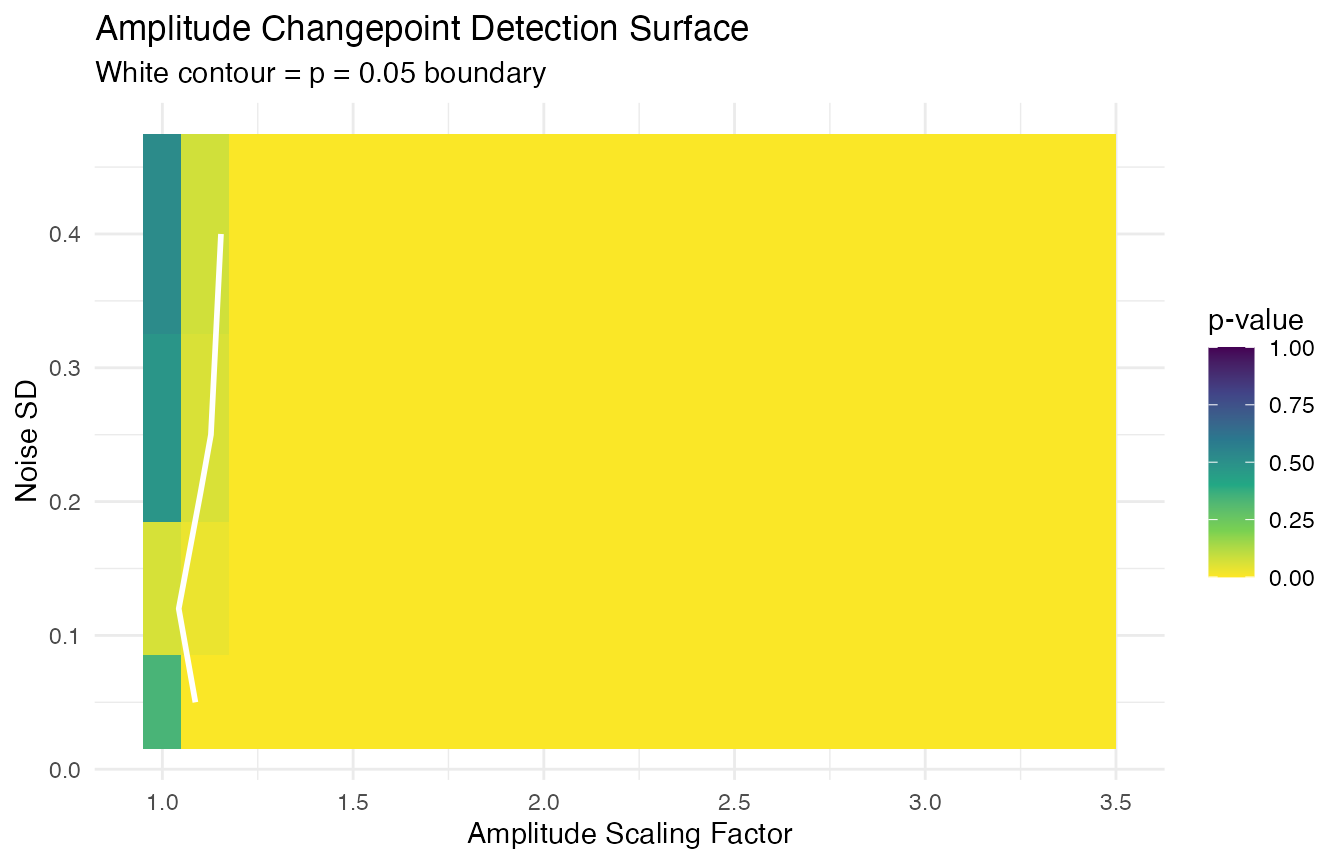

For comparison, here is the 1D slice at the default noise level ($\sigma = 0.12$):

amp_slice <- amp_grid[amp_grid$noise_sd == 0.12, ]

ggplot(amp_slice, aes(x = factor, y = p_value)) +
  geom_line(linewidth = 1) +
  geom_point(size = 3) +
  geom_hline(yintercept = 0.05, linetype = "dashed", color = "#D55E00") +
  annotate("text", x = 2.5, y = 0.08, label = "alpha == 0.05",
           parse = TRUE, color = "#D55E00") +
  scale_y_continuous(limits = c(0, 1)) +
  labs(title = "Amplitude Test at SD = 0.12 (Slice of Surface)",
       x = "Amplitude Scaling Factor",
       y = "Permutation p-value")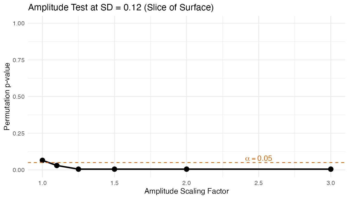

Phase × Noise Surface

We vary the warp strength and noise level. The warp is a Beta CDF $\gamma(t) = F_{\text{Beta}}(t; a, 1/a)$ and the “max deviation” is $\max_t |\gamma(t) - t|$.

warp_strengths <- c(1.0, 1.05, 1.1, 1.2, 1.4, 2.0)

ph_grid <- expand.grid(warp = warp_strengths, noise_sd = noise_sds)
ph_grid$max_dev <- NA_real_
ph_grid$cusum <- NA_real_
ph_grid$p_value <- NA_real_

for (r in seq_len(nrow(ph_grid))) {
  ws <- ph_grid$warp[r]
  sd_val <- ph_grid$noise_sd[r]
  set.seed(42)
  curves_s <- matrix(0, n, m)
  for (i in 1:tau)
    curves_s[i, ] <- template_ph + rnorm(m, sd = sd_val)
  gamma_s <- pbeta(t, ws, 1 / ws)
  ph_grid$max_dev[r] <- max(abs(gamma_s - t))
  for (i in (tau + 1):n)
    curves_s[i, ] <- approx(t, template_ph, xout = gamma_s, rule = 2)$y +
                     rnorm(m, sd = sd_val)
  fd_s <- fdata(curves_s, argvals = t)
  res_s <- elastic.changepoint(fd_s, type = "phase", n.mc = 199, seed = 42)
  ph_grid$cusum[r] <- res_s$test.statistic
  ph_grid$p_value[r] <- res_s$p.value
}

ph_grid <- add_rect_bounds(ph_grid, "warp", "noise_sd")

ggplot(ph_grid, aes(fill = p_value)) +
  geom_rect(aes(xmin = xmin, xmax = xmax, ymin = ymin, ymax = ymax)) +
  geom_contour(aes(x = warp, y = noise_sd, z = p_value), breaks = 0.05,
               color = "white", linewidth = 1) +
  scale_fill_viridis_c(option = "D", direction = -1, limits = c(0, 1),
                       name = "p-value") +
  labs(title = "Phase Changepoint Detection Surface",
       subtitle = "White contour = p = 0.05 boundary",
       x = "Warp Strength", y = "Noise SD") +
  theme(legend.position = "right")
#> Warning: The following aesthetics were dropped during statistical transformation: fill.
#> ℹ This can happen when ggplot fails to infer the correct grouping structure in
#>   the data.
#> ℹ Did you forget to specify a `group` aesthetic or to convert a numerical
#>   variable into a factor?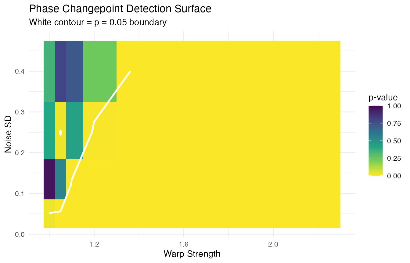

CUSUM Degradation with Noise

Fixing the amplitude factor at 1.5, we see how the CUSUM statistic degrades as noise increases. The test statistic shrinks because the signal is increasingly buried in noise.

noise_sweep <- seq(0.05, 0.5, by = 0.05)
cusum_noise <- data.frame(noise_sd = numeric(), cusum = numeric(),
                          p_value = numeric())

for (sd_val in noise_sweep) {
  set.seed(42)
  curves_s <- matrix(0, n, m)
  for (i in 1:tau)
    curves_s[i, ] <- sin(2 * pi * t) + rnorm(m, sd = sd_val)
  for (i in (tau + 1):n)
    curves_s[i, ] <- 1.5 * sin(2 * pi * t) + 0.5 * 0.4 * sin(4 * pi * t) +
                     rnorm(m, sd = sd_val)
  fd_s <- fdata(curves_s, argvals = t)
  res_s <- elastic.changepoint(fd_s, type = "amplitude", n.mc = 199, seed = 42)
  cusum_noise <- rbind(cusum_noise, data.frame(
    noise_sd = sd_val, cusum = res_s$test.statistic, p_value = res_s$p.value
  ))
}

ggplot(cusum_noise, aes(x = noise_sd, y = cusum)) +
  geom_line(linewidth = 1) +
  geom_point(aes(color = p_value < 0.05), size = 3) +
  scale_color_manual(values = c("TRUE" = "#2166AC", "FALSE" = "#B2182B"),
                     labels = c("TRUE" = "Significant", "FALSE" = "Not significant"),
                     name = "") +
  labs(title = "CUSUM Degradation: Factor = 1.5 Across Noise Levels",
       subtitle = "Test statistic shrinks as noise buries the signal",
       x = "Noise SD", y = "CUSUM Statistic")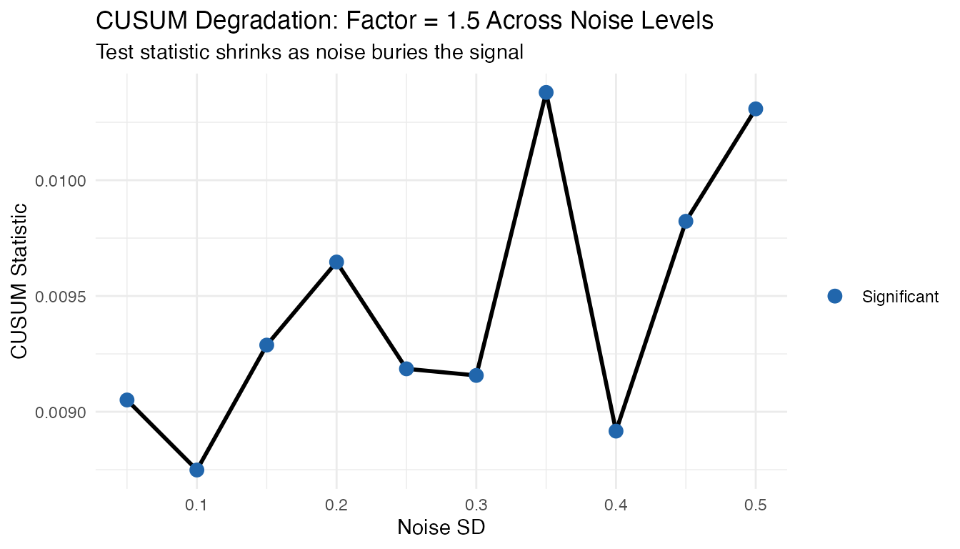

Minimum Detectable Effect

For each noise level, the smallest amplitude factor and warp strength where the test is significant:

# Amplitude: minimum factor per noise level
min_amp_cp <- do.call(rbind, lapply(noise_sds, function(sd_val) {
  sub <- amp_grid[amp_grid$noise_sd == sd_val & amp_grid$factor > 1, ]
  det <- sub$factor[sub$p_value < 0.05]
  data.frame(noise_sd = sd_val,
             min_factor = if (length(det) > 0) min(det) else NA)
}))

# Phase: minimum warp (as max deviation %) per noise level
min_ph_cp <- do.call(rbind, lapply(noise_sds, function(sd_val) {
  sub <- ph_grid[ph_grid$noise_sd == sd_val & ph_grid$warp > 1, ]
  det <- sub[sub$p_value < 0.05, ]
  data.frame(noise_sd = sd_val,
             min_warp_dev = if (nrow(det) > 0)
               paste0(round(min(det$max_dev) * 100, 1), "%") else NA)
}))

mde_cp <- data.frame(
  `Noise SD` = noise_sds,
  `Min Amp Factor` = min_amp_cp$min_factor,
  `Min Warp (max dev %)` = min_ph_cp$min_warp_dev,
  check.names = FALSE
)
knitr::kable(mde_cp, caption = "Minimum detectable effect at alpha = 0.05")

Minimum detectable effect at alpha = 0.05

Noise SD	Min Amp Factor	Min Warp (max dev %)
0.05	1.10	3.4%
0.12	1.10	6.6%
0.25	1.25	3.4%
0.40	1.25	22.8%

Practical Guidance

• Low noise ($\sigma \leq 0.1$): even 10% amplitude changes and 5% temporal displacements are detectable.
• Moderate noise ($\sigma \approx 0.2$): need ~50% amplitude change or ~10% temporal displacement.
• High noise ($\sigma \geq 0.4$): only dramatic changes (2x+ amplitude) are reliably detected.
• Phase detection is inherently more robust: elastic alignment removes amplitude variation before testing, so the phase test is less affected by amplitude noise. This makes it the preferred first test when the noise level is uncertain.

Process Monitoring: Statistical Decision Boundary

For process monitoring applications, a binary OK / Not OK decision requires a statistically valid threshold. The permutation p-value provides exactly this: at significance level $\alpha$, reject $H_0$ (no change) when $p \leq \alpha$.

Setting the Decision Rule

The decision framework works as follows:

1. Collect a calibration set of $n$ functional observations in chronological order during a period of known stable operation.
2. Run elastic.changepoint() with n.mc >= 1000 for a stable p-value.
3. Decision:
   • If $p \leq \alpha$ (e.g., $\alpha = 0.05$): reject $H_0$. A structural change is detected at the estimated $\hat{\tau}$.
   • If $p > \alpha$: do not reject. No significant change detected.

Interpreting the Result

When a changepoint is detected:

What to inspect	How
Where did it happen?	result$changepoint (curve index)
How strong is the change?	Segment L2 effect size (see above)
What kind of change?	Compare amplitude vs phase CUSUM
How confident are we?	result$p.value (smaller = stronger evidence)

Important Considerations

• Multiple testing: If you test the same data with amplitude, phase, and FPCA tests, apply a Bonferroni correction ($\alpha / 3$) or use a single FPCA test as a screening test.
• Sample size: The permutation test has a minimum achievable p-value of $1 / (B + 1)$, where $B$ = n.mc. Use n.mc >= 999 for decisions at $\alpha = 0.05$, and n.mc >= 9999 for $\alpha = 0.01$.
• Prospective monitoring: For ongoing monitoring of a production process, apply the test to a sliding window of the most recent $n$ curves. This provides near-real-time detection of process shifts.

Applications

Elastic changepoint detection is useful whenever a sequence of functional observations may undergo a structural break. The separation of amplitude and phase is the key advantage over classical changepoint methods.

Manufacturing and Quality Control

Sensor profiles from a production line (e.g., temperature curves from a furnace, spectral measurements of output material) can shift when a tool wears out, a raw material batch changes, or a machine is recalibrated.

• Amplitude changepoint: detects when the shape of production curves changes (defective product, drift in process output).
• Phase changepoint: detects when the timing of a process step shifts (e.g., a heating ramp slows down) even if the final product still meets specs.

Biomedicine and Clinical Trials

Longitudinal patient curves (EEG signals, growth trajectories, gait cycles) may change during treatment or disease progression.

• Detect when a patient’s gait pattern changes after surgery (amplitude) or when stride timing shifts (phase).
• In clinical trials, identify the time point at which a drug begins to take effect by monitoring functional biomarker profiles.

Environmental and Climate Monitoring

Seasonal temperature profiles, river discharge curves, or air quality time series may undergo regime changes.

• Amplitude changepoint: identifies when seasonal patterns intensify or weaken (e.g., hotter summers after a climate shift).
• Phase changepoint: identifies when seasons shift in timing (e.g., earlier spring onset due to warming trends).

Speech and Audio Processing

Speaker intonation profiles or phoneme spectrograms may change mid-recording due to emotion, fatigue, or speaker switches.

• Phase changepoints detect changes in speaking rate or rhythm.
• Amplitude changepoints detect changes in pitch contour shape.

Finance

Yield curves, volatility surfaces, or term structure functions observed daily may undergo structural breaks during policy changes or market crises.

Practical Guidance

Use amplitude changepoints for changes in functional shape (quality control, growth curves).

Use phase changepoints for changes in timing (speech patterns, seasonal shifts).

Use FPCA changepoints for changes in principal component structure.

Tips:

• Use n.mc >= 1000 for stable p-values (200 used here for speed)
• Set seed for reproducibility
• Compare CUSUM magnitudes across test types to diagnose the nature of a detected change
• Combine amplitude and phase tests for a complete picture: a process may change in shape, timing, or both

References

• Aue, A. and Horv0e1th, L. (2013). Structural breaks in time series. Journal of Time Series Analysis, 34(1), 1–16.

• Berkes, I., Gabrys, R., Horv0e1th, L. and Kokoszka, P. (2009). Detecting changes in the mean of functional observations. Journal of the Royal Statistical Society: Series B, 71(5), 927–946.

• Srivastava, A., Wu, W., Kurtek, S., Klassen, E. and Marron, J.S. (2011). Registration of functional data using the Fisher-Rao metric. arXiv preprint arXiv:1103.3817.

See Also

• vignette("elastic-alignment") — elastic curve alignment
• vignette("elastic-fpca") — elastic FPCA for amplitude/phase separation
• vignette("streaming-depth") — online monitoring of functional data