Elastic FPCA

Motivation

Functional principal component analysis (FPCA) is a powerful technique for understanding variation in functional data. However, standard FPCA conflates two distinct sources of variation:

Amplitude variability: differences in the values or shape of functions
Phase variability: differences in the timing or alignment of features

Elastic FPCA addresses this by first aligning curves using elastic alignment (via the SRVF framework), then performing FPCA on the aligned curves and warping functions separately.

Elastic FPCA: Separating Amplitude and Phase Variation

Mathematical Framework

The SRVF Representation

Given a function $f : [0,1] \to \mathbb{R}$ , its square-root velocity function (SRVF) is

$q(t) = \text{sign}\bigl(\dot{f}(t)\bigr)\,\sqrt{|\dot{f}(t)|}.$

The key property of the SRVF is that the Fisher-Rao metric between two functions reduces to the $\mathbb{L}^2$ distance between their SRVFs after optimal alignment:

$d_{FR}(f_1, f_2) = \inf_{\gamma \in \Gamma} \|q_1 - (q_2 \circ \gamma)\sqrt{\dot{\gamma}}\|_2,$

where $\Gamma$ is the group of orientation-preserving diffeomorphisms $\gamma : [0,1] \to [0,1]$ .

Karcher Mean

The Karcher mean $\bar{f}$ of a sample $\{f_1,\ldots,f_n\}$ is the Fr0e9chet mean under the Fisher-Rao metric:

$\bar{f} = \arg\min_{f} \sum_{i=1}^{n} d_{FR}(f, f_i)^2.$

The algorithm alternates between (1) aligning each curve to the current mean and (2) computing a new mean from the aligned curves.

Three Modes of FPCA

After computing the Karcher mean, we obtain aligned curves $\{\tilde{f}_i\}$ and warping functions $\{\gamma_i\}$ . These are analyzed with three variants of FPCA:

Vertical (amplitude) FPCA: PCA on the aligned SRVFs $\{\tilde{q}_i\}$ , capturing pure shape variation. The covariance operator is

$C_V(s,t) = \frac{1}{n}\sum_{i=1}^{n} \bigl(\tilde{q}_i(s) - \bar{q}(s)\bigr)\bigl(\tilde{q}_i(t) - \bar{q}(t)\bigr).$

Horizontal (phase) FPCA: PCA on the shooting vectors $v_i = \exp_{\text{id}}^{-1}(\gamma_i)$ in the tangent space at the identity warp, capturing pure timing variation.

Joint FPCA: Concatenates amplitude and phase representations into a combined vector and performs PCA, revealing mixed amplitude-phase modes of variation.

Simulated Data with Amplitude + Phase Variation

n <- 30
m <- 101
t <- seq(0, 1, length.out = m)

# Generate curves with amplitude + phase variation
X <- matrix(0, n, m)
for (i in 1:n) {
  amp <- rnorm(1, 1, 0.3)           # amplitude variation
  shift <- rnorm(1, 0, 0.05)        # phase variation (timing shift)
  X[i, ] <- amp * sin(2 * pi * (t - shift)) +
            0.3 * amp * cos(4 * pi * (t - shift))
}
fd <- fdata(X, argvals = t)

plot(fd, main = "Simulated Curves: Mixed Amplitude + Phase",
     xlab = "t", ylab = "X(t)")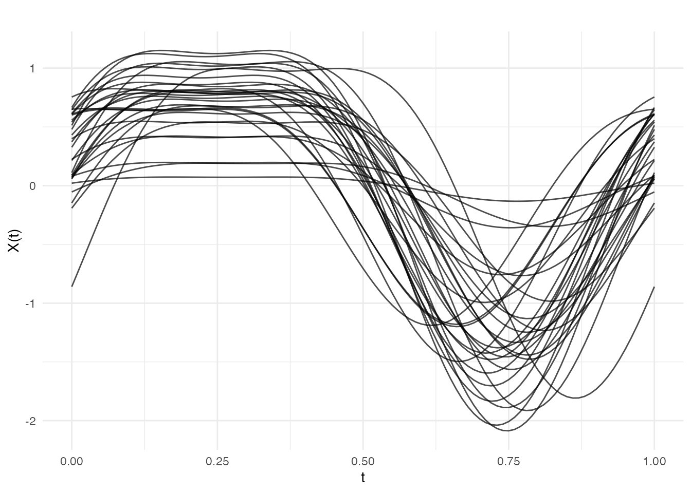

Elastic Alignment

Elastic FPCA begins by aligning curves with karcher.mean():

karcher <- karcher.mean(fd, max.iter = 10)

plot(karcher$aligned, main = "After Elastic Alignment",
     xlab = "t", ylab = "X(t)")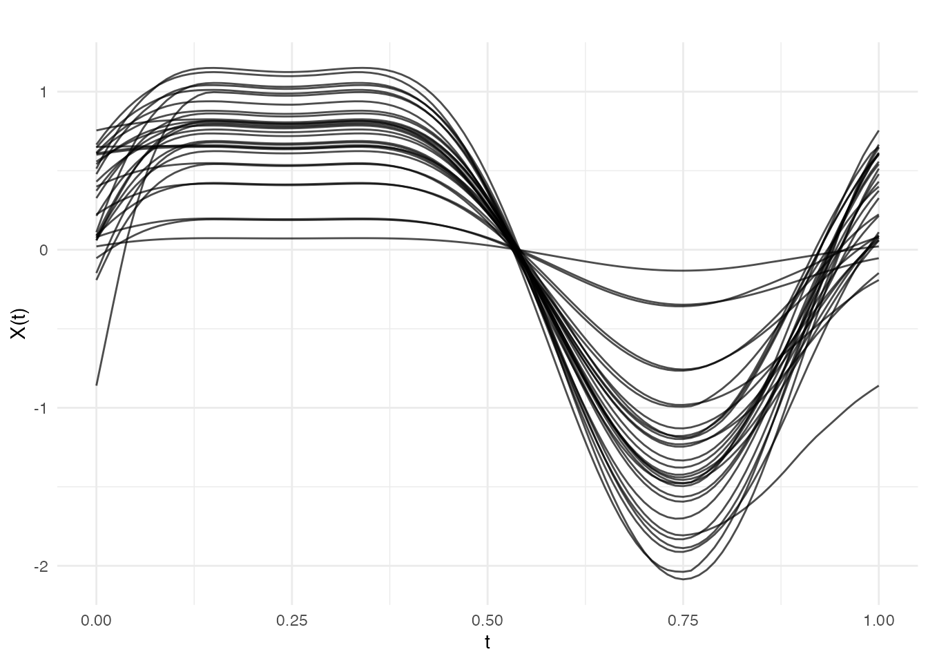

plot(karcher$gammas, main = "Warping Functions (Phase Information)",
     xlab = "t", ylab = expression(gamma(t)))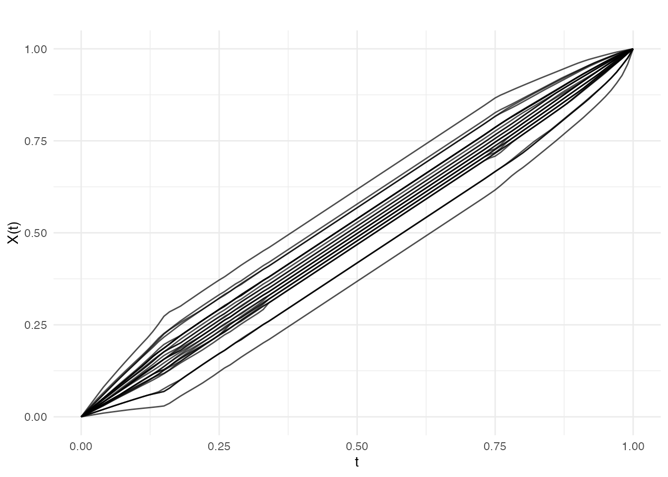

Vertical FPCA: Amplitude Variability

Vertical FPCA performs PCA on the aligned curves, capturing pure shape variation:

vert_result <- vert.fpca(karcher, ncomp = 3)

cat("Vertical FPCA - cumulative variance:\n")
#> Vertical FPCA - cumulative variance:
print(round(vert_result$cumulative.variance, 4))
#> [1] 0.7132 0.9950 1.0000

plot(vert_result, type = "scores")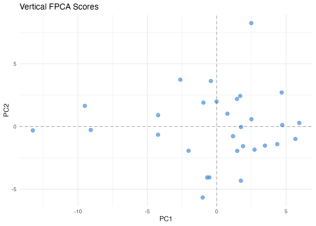

plot(vert_result, type = "eigenfunctions")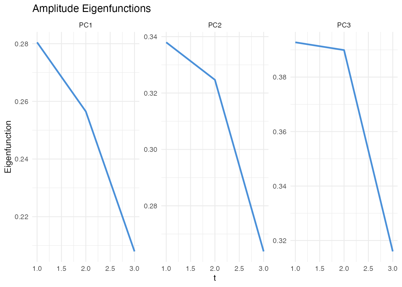

plot(vert_result, type = "variance")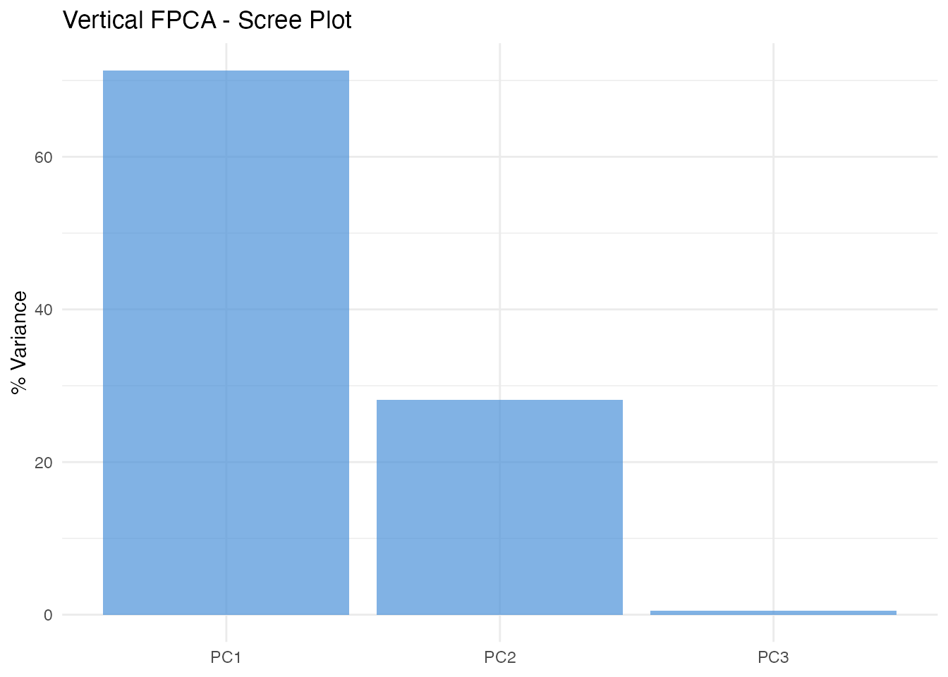

Horizontal FPCA: Phase Variability

Horizontal FPCA analyzes the warping functions, capturing pure timing variation:

horiz_result <- horiz.fpca(karcher, ncomp = 3)

cat("Horizontal FPCA - cumulative variance:\n")
#> Horizontal FPCA - cumulative variance:
print(round(horiz_result$cumulative.variance, 4))
#> [1] 0.9533 0.9817 1.0000

plot(horiz_result, type = "scores")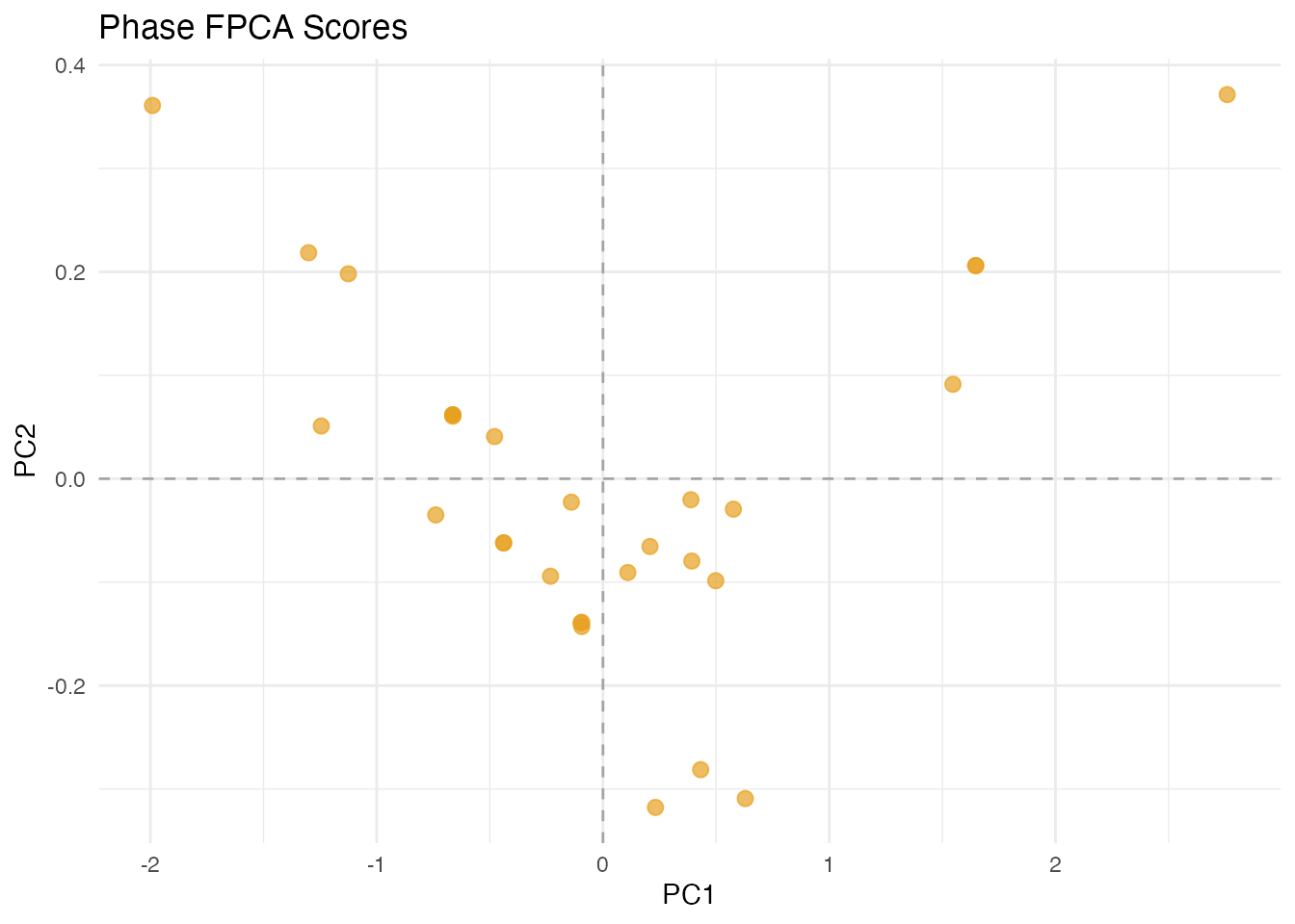

plot(horiz_result, type = "warps")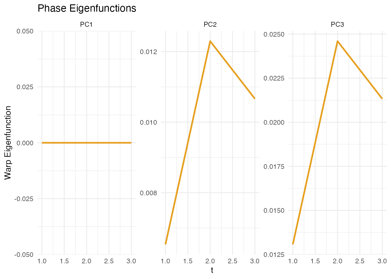

Joint FPCA: Combined Analysis

Joint FPCA simultaneously analyzes both amplitude and phase:

joint_result <- joint.fpca(karcher, ncomp = 3)

cat("Joint FPCA - cumulative variance:\n")
#> Joint FPCA - cumulative variance:
print(round(joint_result$cumulative.variance, 4))
#> [1] 0.7132 0.9950 1.0000

plot(joint_result, type = "scores")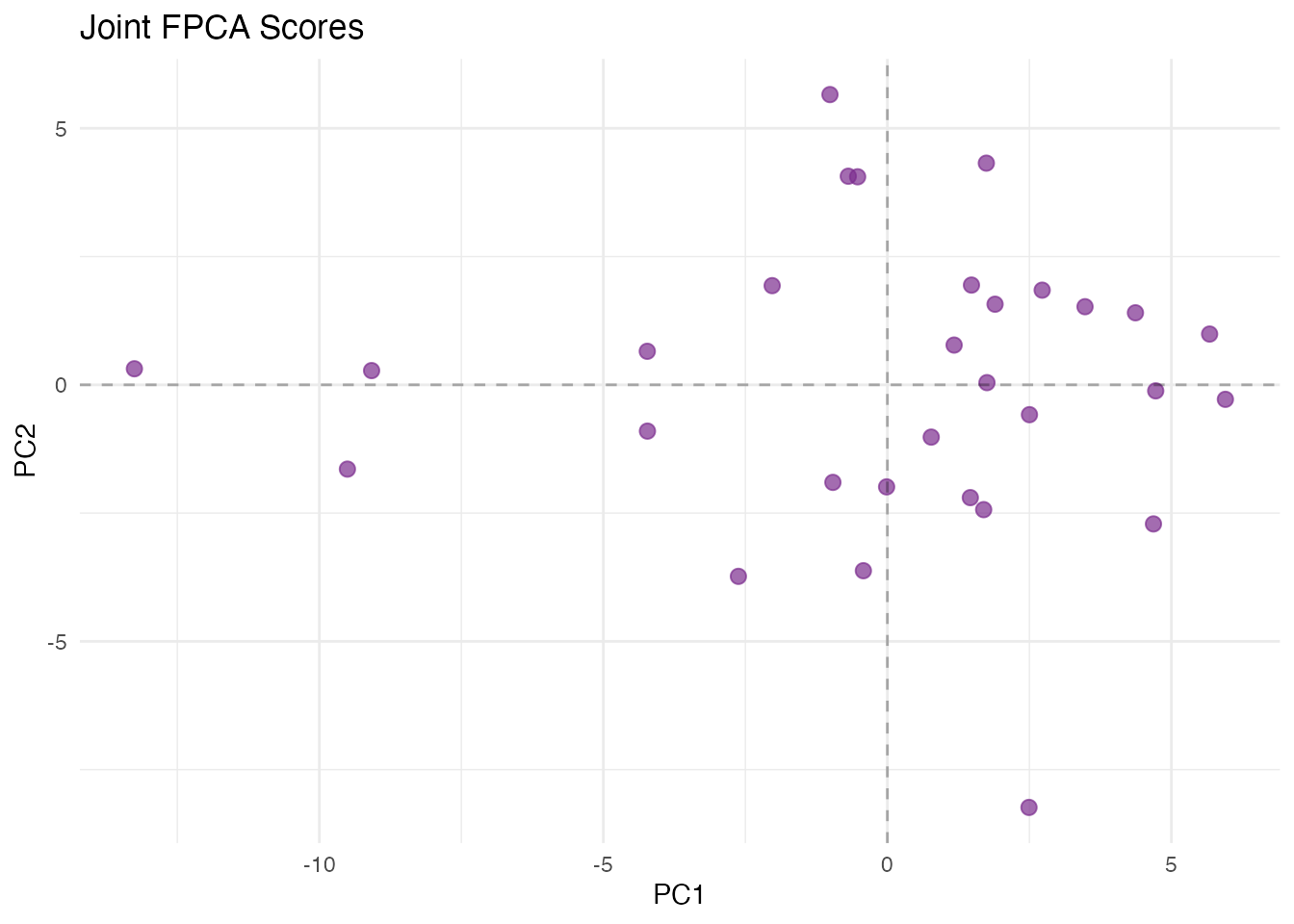

plot(joint_result, type = "balance")
#> Warning in vert_var + horiz_var: longer object length is not a multiple of
#> shorter object length
#> Warning in horiz_var/total: longer object length is not a multiple of shorter
#> object length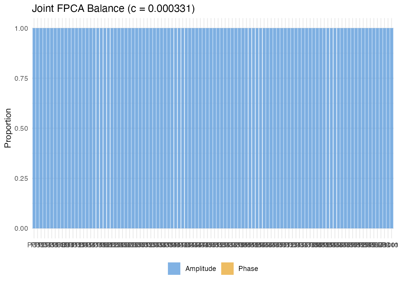

Practical Guidance

Use vertical (amplitude) FPCA when:

You want to understand pure shape variation after removing timing differences

Use horizontal (phase) FPCA when:

You want to understand timing or alignment variation

Use joint FPCA when:

You want to simultaneously analyze amplitude and phase variation
You need to understand their relative contributions

Example applications:

Growth curves: Vertical for shape differences, horizontal for developmental timing
Gait analysis: Vertical for movement patterns, horizontal for stride timing
Weather: Vertical for seasonal temperature patterns, horizontal for seasonal shift

References

Srivastava, A., Wu, W., Kurtek, S., Klassen, E. and Marron, J.S. (2011). Registration of functional data using the Fisher-Rao metric. arXiv preprint arXiv:1103.3817.
Tucker, J.D., Wu, W. and Srivastava, A. (2013). Generative models for functional data using phase and amplitude separation. Computational Statistics & Data Analysis, 61, 50–66.
Srivastava, A. and Klassen, E.P. (2016). Functional and Shape Data Analysis. Springer.
Ramsay, J.O. and Silverman, B.W. (2005). Functional Data Analysis. 2nd ed. Springer.