Functional Equivalence Testing • fdars

Introduction

Classical hypothesis tests (like group.test) ask whether two groups of curves are different. But in many applications the relevant question is the opposite: are two groups of curves equivalent?

Examples include:

Bioequivalence: Do a generic and brand-name drug produce equivalent concentration-time profiles?
Process validation: Does a new manufacturing process produce output curves within tolerance of the old one?
Reproducibility: Do two labs produce equivalent functional measurements?

fequiv.test() implements a functional TOST (Two One-Sided Tests) procedure based on the supremum norm. It constructs a simultaneous confidence band (SCB) for the mean difference and checks whether the entire band lies within an equivalence margin $[-\delta, \delta]$ .

Hypotheses:

$H_0$ : $\sup_t |\mu_1(t) - \mu_2(t)| \geq \delta$ (NOT equivalent)
$H_1$ : $\sup_t |\mu_1(t) - \mu_2(t)| < \delta$ (equivalent)

Setup

library(fdars)
#> 
#> Attaching package: 'fdars'
#> The following objects are masked from 'package:stats':
#> 
#>     cov, decompose, deriv, median, sd, var
#> The following object is masked from 'package:base':
#> 
#>     norm
library(ggplot2)
theme_set(theme_minimal())

set.seed(42)
m <- 100
t_grid <- seq(0, 1, length.out = m)

Example 1: Equivalent curves

Two samples drawn from the same distribution should be declared equivalent with a reasonable $\delta$ .

# Two groups from the same process
n1 <- 30
n2 <- 25
X1 <- matrix(0, n1, m)
X2 <- matrix(0, n2, m)
for (i in 1:n1) X1[i, ] <- sin(2 * pi * t_grid) + rnorm(m, sd = 0.3)
for (i in 1:n2) X2[i, ] <- sin(2 * pi * t_grid) + rnorm(m, sd = 0.3)

fd1 <- fdata(X1, argvals = t_grid)
fd2 <- fdata(X2, argvals = t_grid)

result <- fequiv.test(fd1, fd2, delta = 0.5, n.boot = 1000, seed = 42)
print(result)
#> Functional Equivalence Test (TOST)
#> ===================================
#> Data: fd1 and fd2 
#> Two-sample test, n1 = 30 , n2 = 25 
#> Bootstrap method: multiplier 
#> Equivalence margin (delta): 0.5 
#> Significance level (alpha): 0.05 
#> ---
#> Test statistic (sup|d_hat|): 0.2307 
#> Critical value: 0.0141 
#> SCB range: [ -0.2035 , 0.2448 ]
#> P-value: <2e-16 
#> ---
#> Decision: Reject H0 -- equivalence declared

The plot shows the mean difference curve (black), the simultaneous confidence band (green = equivalence declared, red = not declared), and the equivalence margins (dashed lines at $\pm\delta$ ).

plot(result)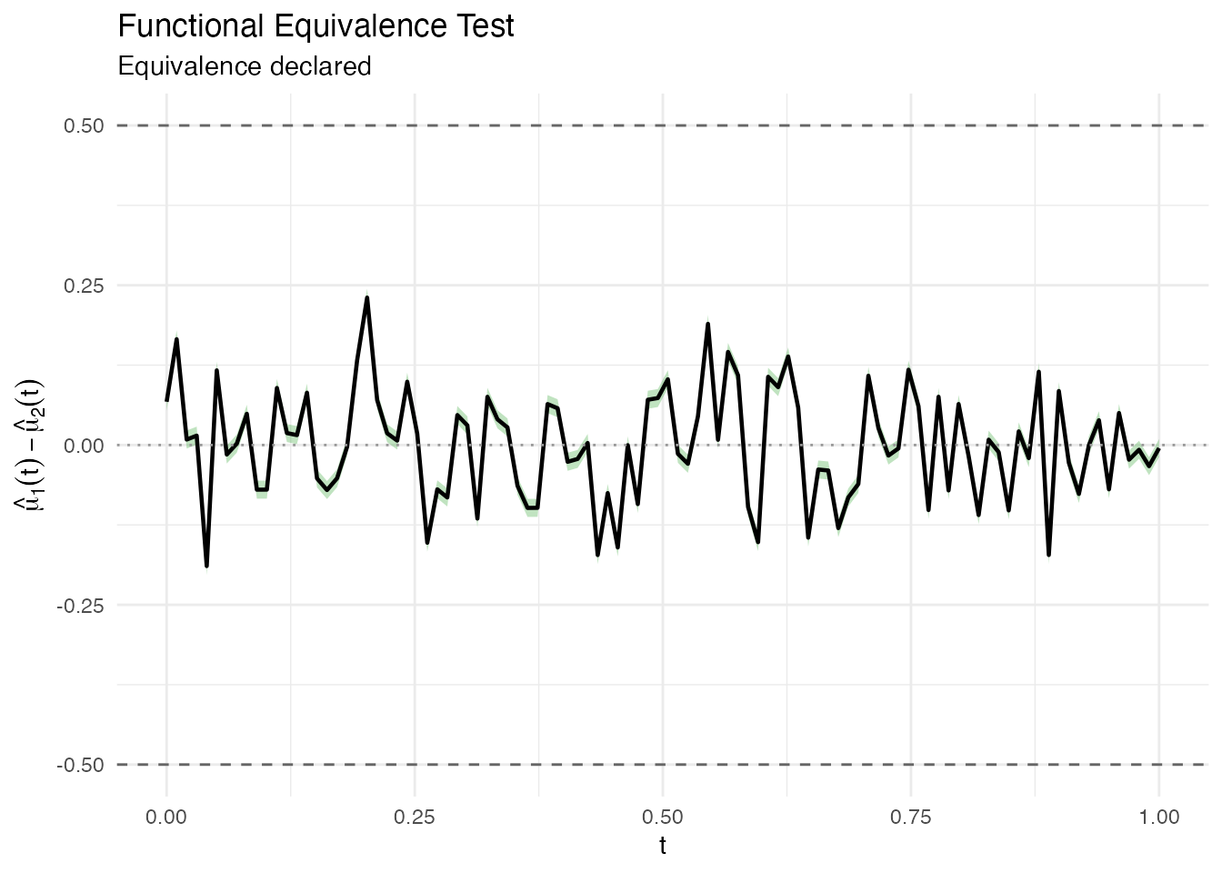

Example 2: Non-equivalent curves

When the two groups have genuinely different mean functions, the test should not declare equivalence.

# Group 2 has a shifted mean
X2_shifted <- matrix(0, n2, m)
for (i in 1:n2) X2_shifted[i, ] <- sin(2 * pi * t_grid) + 0.8 + rnorm(m, sd = 0.3)

fd2_shifted <- fdata(X2_shifted, argvals = t_grid)

result2 <- fequiv.test(fd1, fd2_shifted, delta = 0.5, n.boot = 1000, seed = 42)
print(result2)
#> Functional Equivalence Test (TOST)
#> ===================================
#> Data: fd1 and fd2_shifted 
#> Two-sample test, n1 = 30 , n2 = 25 
#> Bootstrap method: multiplier 
#> Equivalence margin (delta): 0.5 
#> Significance level (alpha): 0.05 
#> ---
#> Test statistic (sup|d_hat|): 0.9969 
#> Critical value: 0.014 
#> SCB range: [ -1.0109 , -0.5899 ]
#> P-value: 1 
#> ---
#> Decision: Fail to reject H0 -- equivalence NOT declared

plot(result2)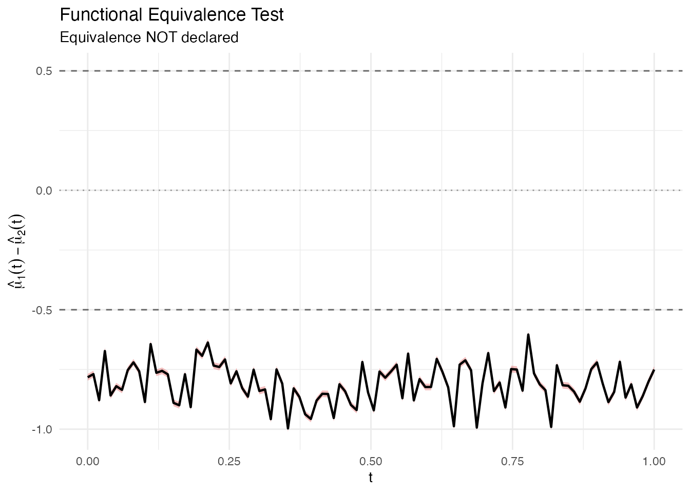

The red band extends well beyond the dashed equivalence margins, so equivalence is not declared.

Choosing delta

The equivalence margin $\delta$ is the maximum sup-norm difference you consider scientifically negligible. It must be chosen before looking at the data, based on domain knowledge:

Too large: trivially declares equivalence (low power against real differences)
Too small: almost never declares equivalence (conservative)

A useful diagnostic is to sweep over $\delta$ values and see where the decision flips:

deltas <- seq(0.1, 1.0, by = 0.05)
decisions <- sapply(deltas, function(d) {
  fequiv.test(fd1, fd2, delta = d, n.boot = 500, seed = 42)$reject
})

df_sweep <- data.frame(delta = deltas, equivalent = decisions)
ggplot(df_sweep, aes(x = delta, y = as.numeric(equivalent))) +
  geom_step(linewidth = 0.8) +
  geom_point(aes(color = equivalent), size = 2) +
  scale_color_manual(values = c("FALSE" = "#d62728", "TRUE" = "#2ca02c")) +
  labs(x = expression(delta), y = "Equivalence declared",
       title = "Decision as a function of equivalence margin") +
  scale_y_continuous(breaks = c(0, 1), labels = c("No", "Yes"))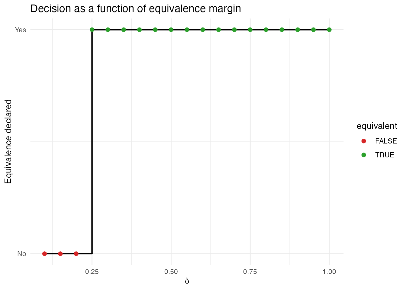

One-sample test

You can also test whether a single sample’s mean is equivalent to a known reference function $\mu_0$ .

# Test if the sample mean is equivalent to the true generating function
mu0 <- sin(2 * pi * t_grid)
result_one <- fequiv.test(fd1, delta = 0.5, mu0 = mu0, n.boot = 1000, seed = 42)
print(result_one)
#> Functional Equivalence Test (TOST)
#> ===================================
#> Data: fd1 
#> One-sample test, n = 30 
#> Bootstrap method: multiplier 
#> Equivalence margin (delta): 0.5 
#> Significance level (alpha): 0.05 
#> ---
#> Test statistic (sup|d_hat|): 0.1243 
#> Critical value: 0.0061 
#> SCB range: [ -0.1305 , 0.1088 ]
#> P-value: <2e-16 
#> ---
#> Decision: Reject H0 -- equivalence declared
plot(result_one)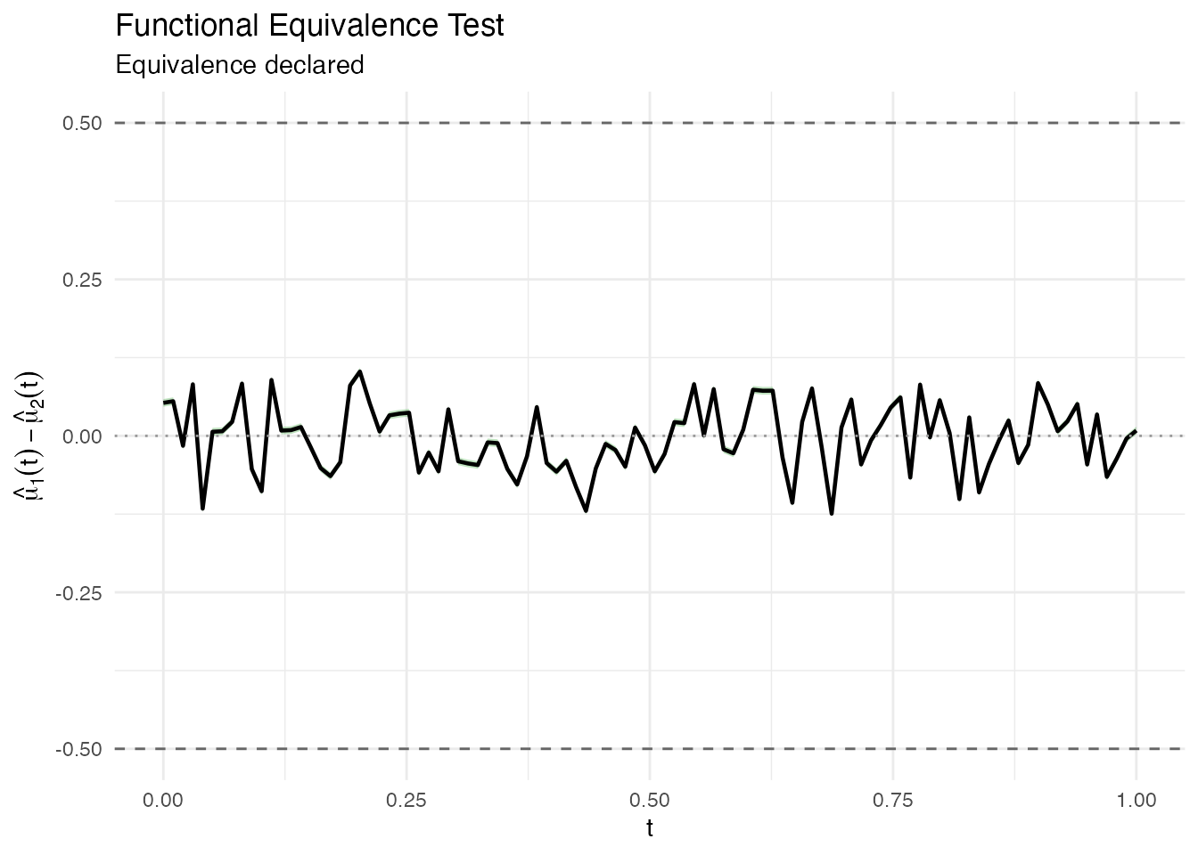

Bootstrap methods

fequiv.test supports two bootstrap methods:

"multiplier" (default): Gaussian multiplier bootstrap. Fast and asymptotically valid. Recommended for most applications.
"percentile": Resampling-based bootstrap. More robust with small samples or heavy-tailed data.

result_pct <- fequiv.test(fd1, fd2, delta = 0.5, n.boot = 1000,
                          method = "percentile", seed = 42)
print(result_pct)
#> Functional Equivalence Test (TOST)
#> ===================================
#> Data: fd1 and fd2 
#> Two-sample test, n1 = 30 , n2 = 25 
#> Bootstrap method: percentile 
#> Equivalence margin (delta): 0.5 
#> Significance level (alpha): 0.05 
#> ---
#> Test statistic (sup|d_hat|): 0.2307 
#> Critical value: 0.2691 
#> SCB range: [ -0.4585 , 0.4998 ]
#> P-value: 0.1 
#> ---
#> Decision: Reject H0 -- equivalence declared

References

Dette, H. and Kokot, K. (2021). Detecting relevant differences in the covariance operators of functional time series. Biometrika, 108(4):895–913.