Berkeley Growth Study: Elastic Alignment of Growth Velocity
Source:vignettes/articles/example-berkeley-growth.Rmd
example-berkeley-growth.Rmd93 children’s growth velocity curves (ages 1–18) are elastically aligned to separate when each child’s growth spurt occurs from how tall it is.
| Step | What It Does | Outcome |
|---|---|---|
| Elastic alignment | Remove timing differences across children | Variance reduction of ~60% in pubertal region; de-blurred Karcher mean recovers true peak shape |
| Warping functions | Extract per-child maturation timing | Scalar “timing shift” score per child, usable as a covariate in downstream regression |
| Equivalence test | Test whether boys and girls differ in timing | Equivalence rejected at years — ~2 year gap confirmed with bootstrap CIs |
| FPCA on warpings | Identify main modes of timing variation | PC1 (83%) separates boys from girls; PC2 captures secondary timing structure |
Key result: Girls’ pubertal growth spurt peaks ~2 years earlier than boys’ (mean age 11.5 vs 13.5). The warping functions quantify this precisely for each child and can be correlated with other variables (adult height, BMI, etc.).
This dataset is a standard benchmark in elastic FDA literature
(Tucker et al., 2013; Srivastava and Klassen, 2016). It is available in
the fdasrvf package.
Data Preparation
data(growth_vel, package = "fdasrvf")

# growth_vel$f is 69 (grid) x 93 (curves) — transpose for fdata
# Standard ordering: first 39 = boys, last 54 = girls
fd_growth_raw <- fdata(t(growth_vel$f), argvals = growth_vel$time)
gender <- factor(c(rep("Boy", 39), rep("Girl", 54)))
cat("Curves:", nrow(fd_growth_raw$data),
    "(", sum(gender == "Boy"), "boys,", sum(gender == "Girl"), "girls)\n")
#> Curves: 93 ( 39 boys, 54 girls)
cat("Grid points:", ncol(fd_growth_raw$data), "\n")
#> Grid points: 69
cat("Age range:", range(fd_growth_raw$argvals), "\n")
#> Age range: 1 18
The raw data has only 69 grid points, which is coarse for elastic alignment (the DP warping resolution is limited). We smooth with P-splines and evaluate on a finer grid:
# Smooth with P-splines and evaluate on a finer grid
fine_argvals <- seq(min(fd_growth_raw$argvals), max(fd_growth_raw$argvals),
                    length.out = 200)
coefs_growth <- fdata2basis(fd_growth_raw, nbasis = 25, type = "bspline")
fd_growth <- basis2fdata(coefs_growth, fine_argvals)
cat("Smoothed grid points:", ncol(fd_growth$data), "\n")
#> Smoothed grid points: 200
Full Age Range
plot(fd_growth) + labs(title = "Berkeley Growth Velocity (all 93 children)",
                       x = "Age (years)", y = "Growth velocity (cm/year)")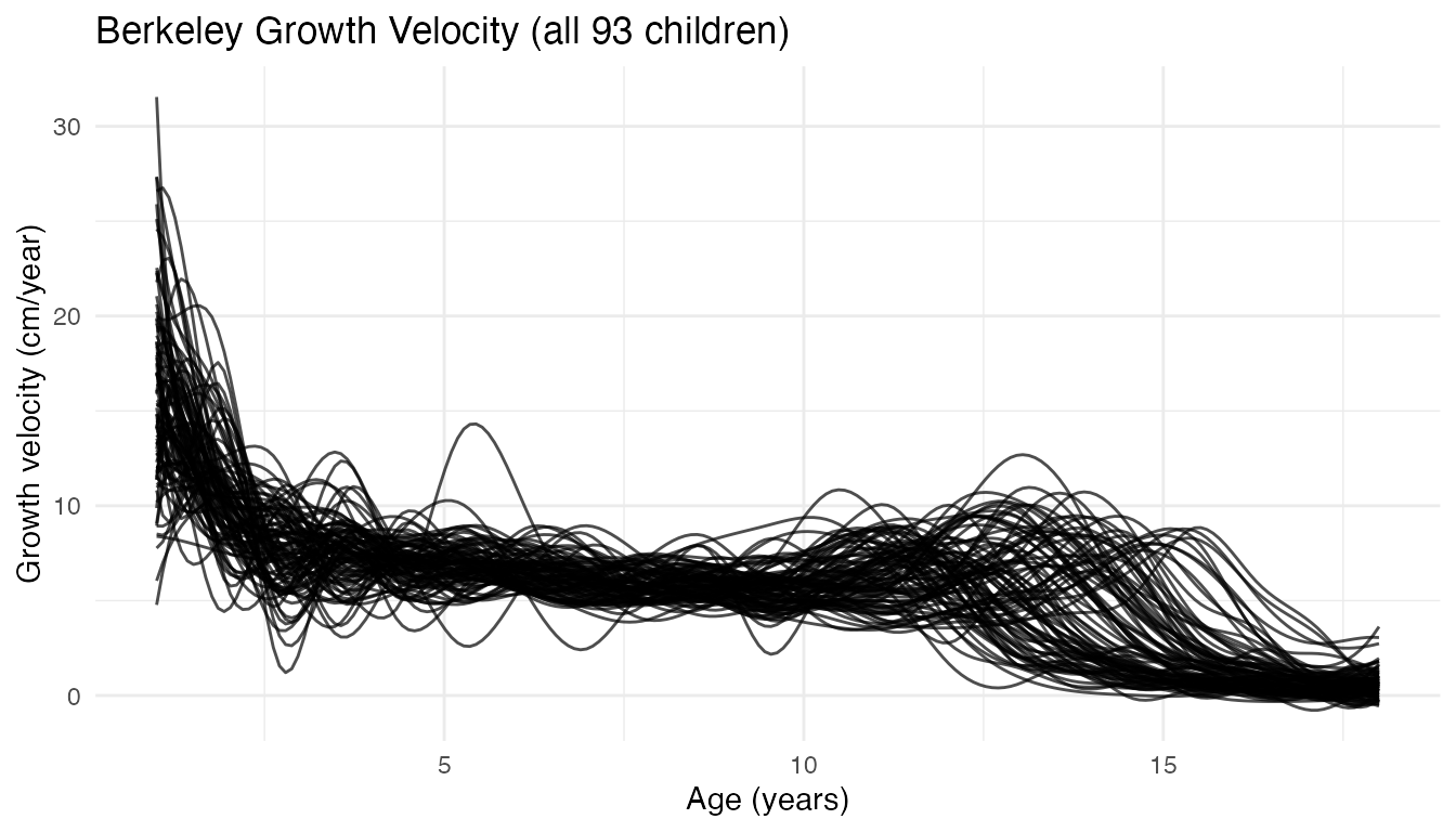
The dominant feature at age 1 (infant growth) and the pubertal spurt around ages 11–14 are both visible, but the pubertal peak is blurred by phase variability.
res_growth <- elastic.align(fd_growth)
var_orig_growth <- mean(apply(fd_growth$data, 2, var))
vr_growth <- 1 - mean(apply(res_growth$aligned$data, 2, var)) / var_orig_growth
cat("Full range VR:", round(vr_growth * 100, 1), "%\n")
#> Full range VR: 48.6 %
plot(res_growth, type = "both")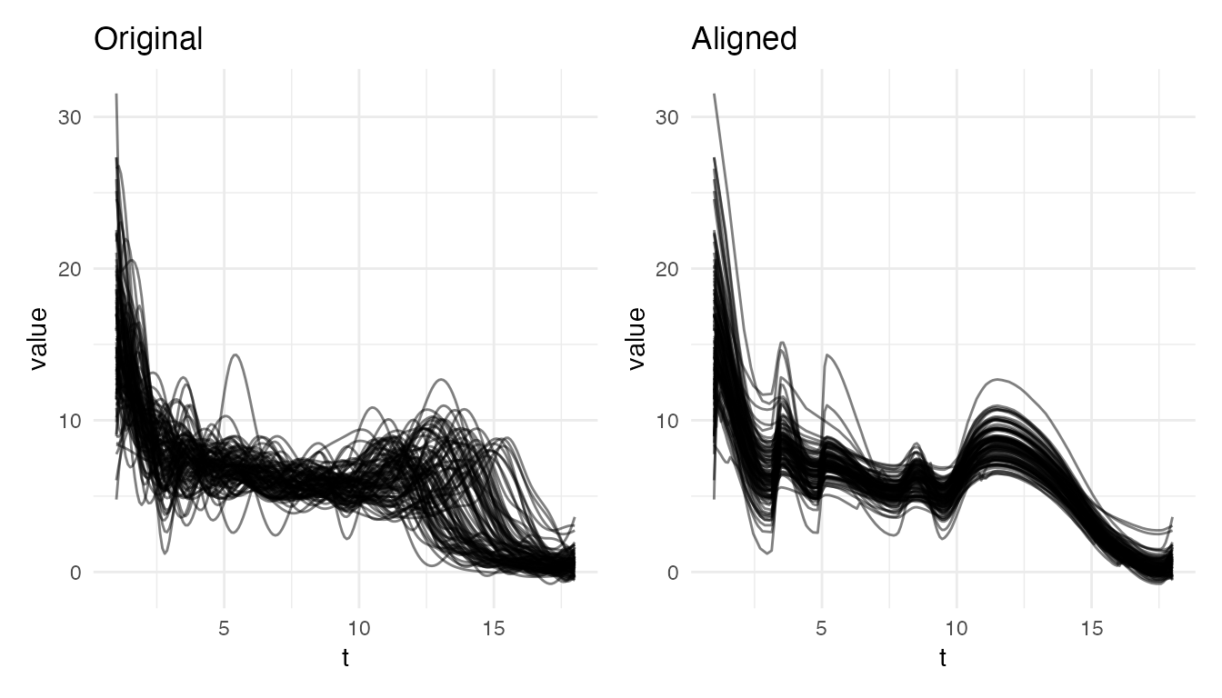
Pubertal Growth Spurt (Ages 8–18)
The pubertal region is where phase variability is strongest. Restricting to ages 8–18 isolates the growth spurt:
idx_pub <- which(fd_growth$argvals >= 8)
fd_pub <- fdata(fd_growth$data[, idx_pub],
                argvals = fd_growth$argvals[idx_pub])

res_pub <- elastic.align(fd_pub)
var_pub <- mean(apply(fd_pub$data, 2, var))
vr_pub <- 1 - mean(apply(res_pub$aligned$data, 2, var)) / var_pub
cat("Pubertal region VR:", round(vr_pub * 100, 1), "%\n")
#> Pubertal region VR: 77.7 %
plot(res_pub, type = "both")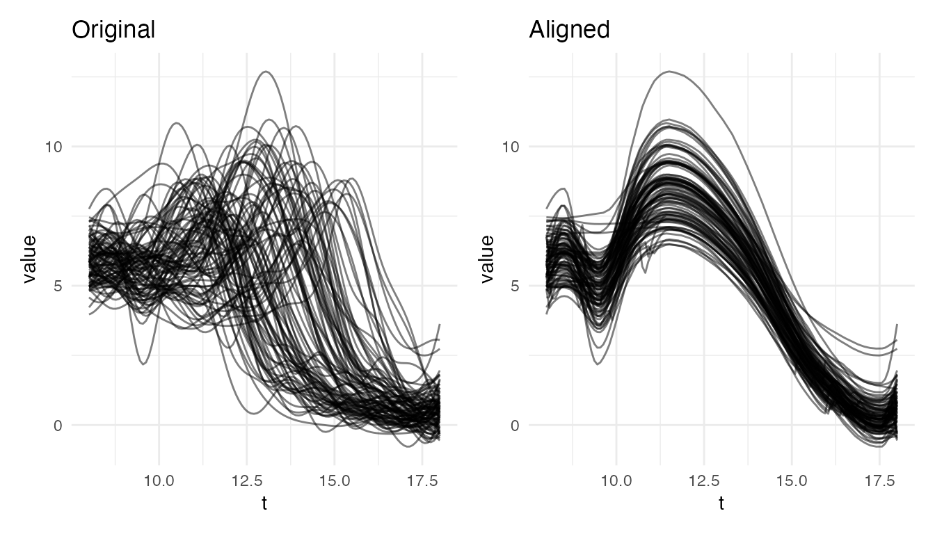
Cross-Sectional Mean vs Karcher Mean
The Karcher mean serves as the reference frame that gives the warping functions their meaning – each is defined as “warp curve to match this mean.” Without a consistent reference, the warpings would not be comparable across children.
As a bonus, the Karcher mean also recovers a de-blurred population average. The cross-sectional mean is attenuated because children’s growth spurts are averaged at mismatched ages; the Karcher mean recovers the true peak amplitude:
km_pub <- karcher.mean(fd_pub, max.iter = 20)
cross_mean_pub <- as.numeric(mean(fd_pub)$data)
karcher_pub <- as.numeric(km_pub$mean$data)

cat("Cross-sectional mean peak:", round(max(cross_mean_pub), 2), "cm/yr at age",
    round(fd_pub$argvals[which.max(cross_mean_pub)], 1), "\n")
#> Cross-sectional mean peak: 6.39 cm/yr at age 11.5
cat("Karcher mean peak:        ", round(max(karcher_pub), 2), "cm/yr at age",
    round(fd_pub$argvals[which.max(karcher_pub)], 1), "\n")
#> Karcher mean peak:         8.44 cm/yr at age 12.4
df_means <- data.frame(
  age = rep(fd_pub$argvals, 2),
  velocity = c(cross_mean_pub, karcher_pub),
  type = rep(c("Cross-sectional mean", "Karcher mean"),
             each = length(fd_pub$argvals))
)

ggplot(df_means, aes(x = age, y = velocity, color = type)) +
  geom_line(linewidth = 1.2) +
  scale_color_manual(values = c("Cross-sectional mean" = "steelblue",
                                "Karcher mean" = "firebrick")) +
  labs(title = "Pubertal Growth Spurt: Cross-Sectional vs Karcher Mean",
       x = "Age (years)", y = "Growth velocity (cm/year)", color = NULL)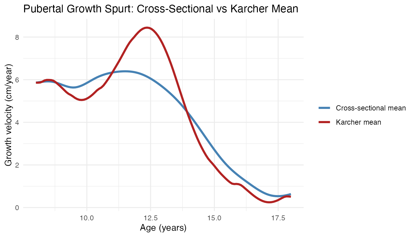
The Karcher mean is sharper and taller because it aligns the growth spurts before averaging, rather than smearing them across different ages. This sharper shape is a better estimate of the typical growth velocity profile – but its primary role is as the anchor that makes the per-child warping functions interpretable and mutually comparable.
FPCA Before and After Alignment
Alignment concentrates variance into fewer principal components:
pc_before <- fdata2pc(fd_pub, ncomp = 3)
pc_after <- fdata2pc(km_pub$aligned, ncomp = 3)

pve_before <- round(pc_before$d^2 / sum(pc_before$d^2) * 100, 1)
pve_after <- round(pc_after$d^2 / sum(pc_after$d^2) * 100, 1)

cat("Before alignment: PC1 =", pve_before[1], "%, PC2 =", pve_before[2],
    "%, PC3 =", pve_before[3], "%\n")
#> Before alignment: PC1 = 67.6 %, PC2 = 26.3 %, PC3 = 6.1 %
cat("After alignment:  PC1 =", pve_after[1], "%, PC2 =", pve_after[2],
    "%, PC3 =", pve_after[3], "%\n")
#> After alignment:  PC1 = 57.6 %, PC2 = 32.3 %, PC3 = 10.1 %
Before alignment, phase variability spreads across multiple PCs. After alignment, the remaining (amplitude) variability is more efficiently captured by the first PC.
Warping Functions Reveal Growth Timing
The warping functions are the main extracted quantity from this analysis. Each maps population-average time to child ’s biological time, revealing how their developmental clock differs from the Karcher mean reference:
n_pub <- nrow(res_pub$gammas$data)
m_pub <- ncol(res_pub$gammas$data)
df_warps <- data.frame(
  t = rep(res_pub$gammas$argvals, n_pub),
  gamma = as.vector(t(res_pub$gammas$data)),
  curve = rep(seq_len(n_pub), each = m_pub),
  sex = rep(gender, each = m_pub)
)

ggplot(df_warps, aes(x = t, y = gamma, group = curve, color = sex)) +
  geom_abline(slope = 1, intercept = 0, linetype = "dashed", color = "grey60") +
  geom_line(alpha = 0.4) +
  scale_color_manual(values = c(Boy = "steelblue", Girl = "coral")) +
  labs(title = "Warping Functions by Sex",
       x = "Reference age (years)",
       y = expression(gamma(t)), color = NULL) +
  theme(legend.position = "top")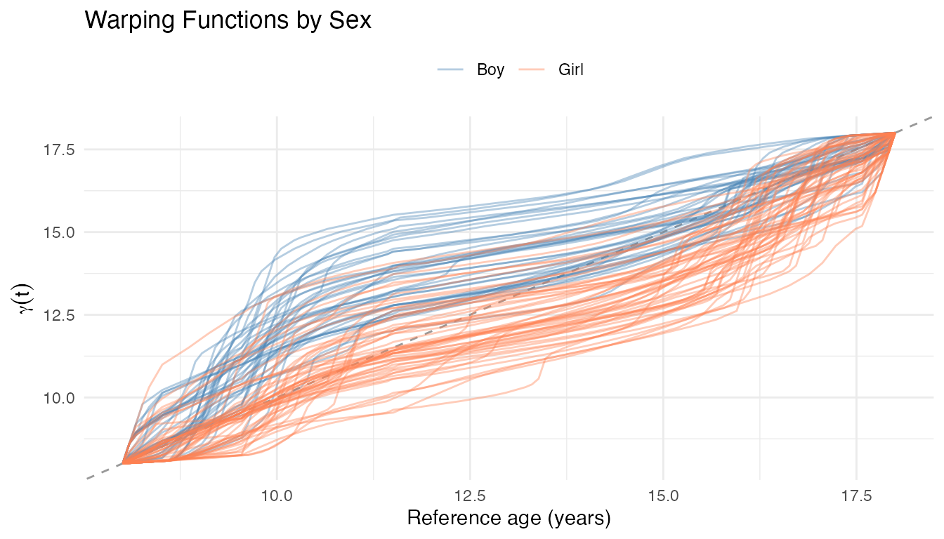
Each maps from the reference time axis (the Karcher mean) to the corresponding age in child ’s original curve. Curves below the diagonal () indicate that the growth spurt occurred at a younger age than the population average – i.e., earlier maturation. Curves above the diagonal indicate later maturation.
The colour separation confirms the well-known pattern: girls (coral) cluster below the diagonal, reflecting earlier pubertal timing, while boys (blue) cluster above.
Testing the Gender Difference in Timing
The visual pattern suggests boys and girls differ in pubertal timing.
We can test this formally with fequiv.test(), which checks
whether the mean warping functions of two groups are equivalent within a
margin
.
If equivalence is not declared, we have evidence the timing
patterns genuinely differ.
We use years – differences smaller than half a year would be considered practically negligible:
warps_boys <- km_pub$gammas[gender == "Boy"]
warps_girls <- km_pub$gammas[gender == "Girl"]

set.seed(42)
equiv <- fequiv.test(warps_boys, warps_girls, delta = 0.5,
                     n.boot = 1000, seed = 42)
print(equiv)
#> Functional Equivalence Test (TOST)
#> ===================================
#> Data: warps_boys and warps_girls
#> Two-sample test, n1 = 39 , n2 = 54
#> Bootstrap method: multiplier
#> Equivalence margin (delta): 0.5
#> Significance level (alpha): 0.05
#> ---
#> Test statistic (sup|d_hat|): 2.0033
#> Critical value: 0.4225
#> SCB range: [ -0.4225 , 2.4258 ]
#> P-value: 1
#> ---
#> Decision: Fail to reject H0 -- equivalence NOT declared
plot(equiv) +
  labs(x = "Age (years)",
       y = expression(hat(gamma)[boys](t) - hat(gamma)[girls](t)))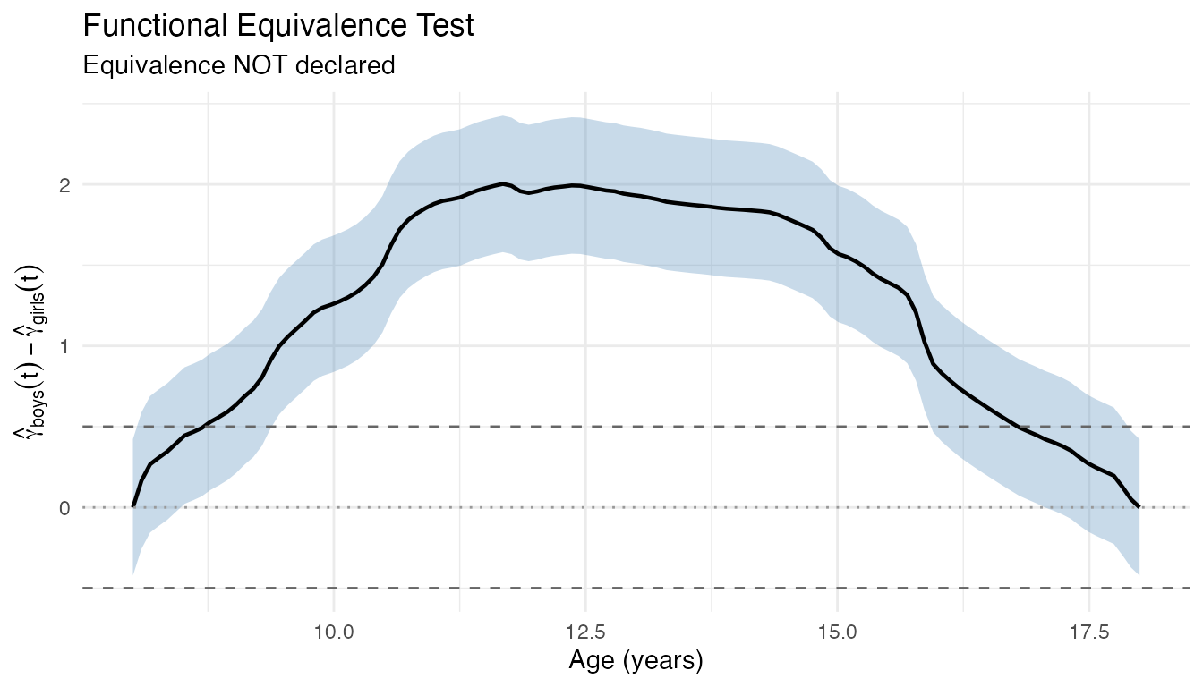
The mean difference curve (solid line) and its simultaneous confidence band (shaded) both far exceed the year margins (dashed lines), so equivalence is decisively rejected.
The mean warping functions for each group show the separation directly:
t_pub <- warps_boys$argvals
mean_warp_boys <- as.numeric(mean(warps_boys)$data)
mean_warp_girls <- as.numeric(mean(warps_girls)$data)

# Pointwise 95% CI via bootstrap
set.seed(42)
n_boot <- 1000
boot_boys <- matrix(0, n_boot, length(t_pub))
boot_girls <- matrix(0, n_boot, length(t_pub))
for (b in seq_len(n_boot)) {
  boot_boys[b, ] <- colMeans(warps_boys$data[sample(nrow(warps_boys$data),
                              replace = TRUE), ])
  boot_girls[b, ] <- colMeans(warps_girls$data[sample(nrow(warps_girls$data),
                               replace = TRUE), ])
}
ci_boys_lo <- apply(boot_boys, 2, quantile, 0.025)
ci_boys_hi <- apply(boot_boys, 2, quantile, 0.975)
ci_girls_lo <- apply(boot_girls, 2, quantile, 0.025)
ci_girls_hi <- apply(boot_girls, 2, quantile, 0.975)

df_ci <- rbind(
  data.frame(t = t_pub, lo = ci_boys_lo, hi = ci_boys_hi, group = "Boys"),
  data.frame(t = t_pub, lo = ci_girls_lo, hi = ci_girls_hi, group = "Girls")
)
df_mean_warps <- data.frame(
  t = rep(t_pub, 3),
  gamma = c(mean_warp_boys, mean_warp_girls, t_pub),
  group = rep(c("Boys", "Girls", "Identity"), each = length(t_pub))
)

ggplot() +
  geom_ribbon(data = df_ci, aes(x = t, ymin = lo, ymax = hi, fill = group),
              alpha = 0.2) +
  geom_line(data = df_mean_warps,
            aes(x = t, y = gamma, color = group, linetype = group),
            linewidth = 1) +
  geom_abline(slope = 1, intercept = 0, linetype = "dashed", color = "grey60") +
  scale_color_manual(values = c(Boys = "steelblue", Girls = "coral",
                                Identity = "grey60")) +
  scale_fill_manual(values = c(Boys = "steelblue", Girls = "coral")) +
  scale_linetype_manual(values = c(Boys = "solid", Girls = "solid",
                                   Identity = "dashed")) +
  labs(title = "Mean Warping Functions by Sex (95% CI)",
       x = "Reference age (years)", y = expression(bar(gamma)(t)),
       color = NULL, linetype = NULL, fill = NULL) +
  guides(fill = "none") +
  theme(legend.position = "top")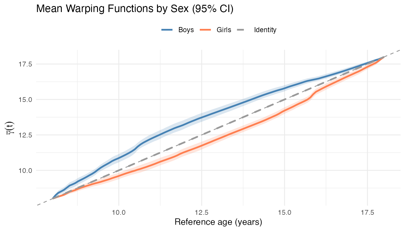
Girls’ mean warping sits below the identity (the growth spurt features occur at younger ages), while boys’ sits above. The vertical gap between the two curves represents the timing difference at each reference age.
We can quantify the timing gap directly from the original curves:
peak_ages <- fd_pub$argvals[apply(fd_pub$data, 1, which.max)]
cat("Boys: mean peak age =", round(mean(peak_ages[gender == "Boy"]), 1),
    "years (sd =", round(sd(peak_ages[gender == "Boy"]), 1), ")\n")
#> Boys: mean peak age = 13.5 years (sd = 1.3 )
cat("Girls: mean peak age =", round(mean(peak_ages[gender == "Girl"]), 1),
    "years (sd =", round(sd(peak_ages[gender == "Girl"]), 1), ")\n")
#> Girls: mean peak age = 11.4 years (sd = 1.3 )
cat("Difference:", round(mean(peak_ages[gender == "Boy"]) -
    mean(peak_ages[gender == "Girl"]), 1), "years\n")
#> Difference: 2.1 years
The equivalence test on the warping functions confirms what the peak ages show: boys and girls have meaningfully different growth timing.
Working with Warping Functions
The warping functions
are fdata objects, so they can be used with any fdars
function. Here are concrete ways to extract information from them:
Scalar summaries per child. The deviation from the identity summarises how much each child’s timing differs from the reference. Averaging this gives a single “timing shift” score per child:
# Timing shift: mean deviation from identity (positive = later, negative = earlier)
t_pub <- km_pub$gammas$argvals
identity <- matrix(t_pub, nrow = nrow(km_pub$gammas$data),
                   ncol = length(t_pub), byrow = TRUE)
timing_shift <- rowMeans(km_pub$gammas$data - identity)

cat("Earliest maturer: child", which.min(timing_shift),
    "(shift =", round(min(timing_shift), 2), "years)\n")
#> Earliest maturer: child 42 (shift = -1.82 years)
cat("Latest maturer:   child", which.max(timing_shift),
    "(shift =", round(max(timing_shift), 2), "years)\n")
#> Latest maturer:   child 27 (shift = 1.92 years)
These scalar scores can be used as covariates in standard regression, or for correlation with other variables (e.g., adult height, BMI):
df_shift <- data.frame(shift = timing_shift, sex = gender)
ggplot(df_shift, aes(x = sex, y = shift, fill = sex)) +
  geom_boxplot(alpha = 0.6, outlier.shape = 21) +
  geom_hline(yintercept = 0, linetype = "dashed", color = "grey50") +
  scale_fill_manual(values = c(Boy = "steelblue", Girl = "coral")) +
  labs(title = "Timing Shift Scores by Sex",
       x = NULL, y = "Mean timing shift (years)") +
  guides(fill = "none")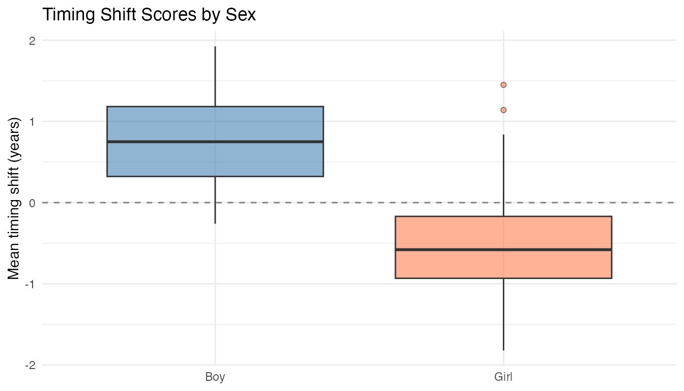
FPCA on warping functions. The warpings themselves can be analysed as functional data. Functional PCA on the warping functions identifies the main modes of timing variation:
pc_warps <- fdata2pc(km_pub$gammas, ncomp = 2)
pve_warps <- round(pc_warps$d^2 / sum(pc_warps$d^2) * 100, 1)
cat("Warp PC1:", pve_warps[1], "% — PC2:", pve_warps[2], "%\n")
#> Warp PC1: 91.8 % — PC2: 8.2 %
df_scores <- data.frame(
  PC1 = pc_warps$x[, 1],
  PC2 = pc_warps$x[, 2],
  sex = gender
)
ggplot(df_scores, aes(x = PC1, y = PC2, color = sex)) +
  geom_point(size = 2, alpha = 0.7) +
  scale_color_manual(values = c(Boy = "steelblue", Girl = "coral")) +
  labs(title = "PCA of Warping Functions",
       x = paste0("PC1 (", pve_warps[1], "%)"),
       y = paste0("PC2 (", pve_warps[2], "%)"),
       color = NULL)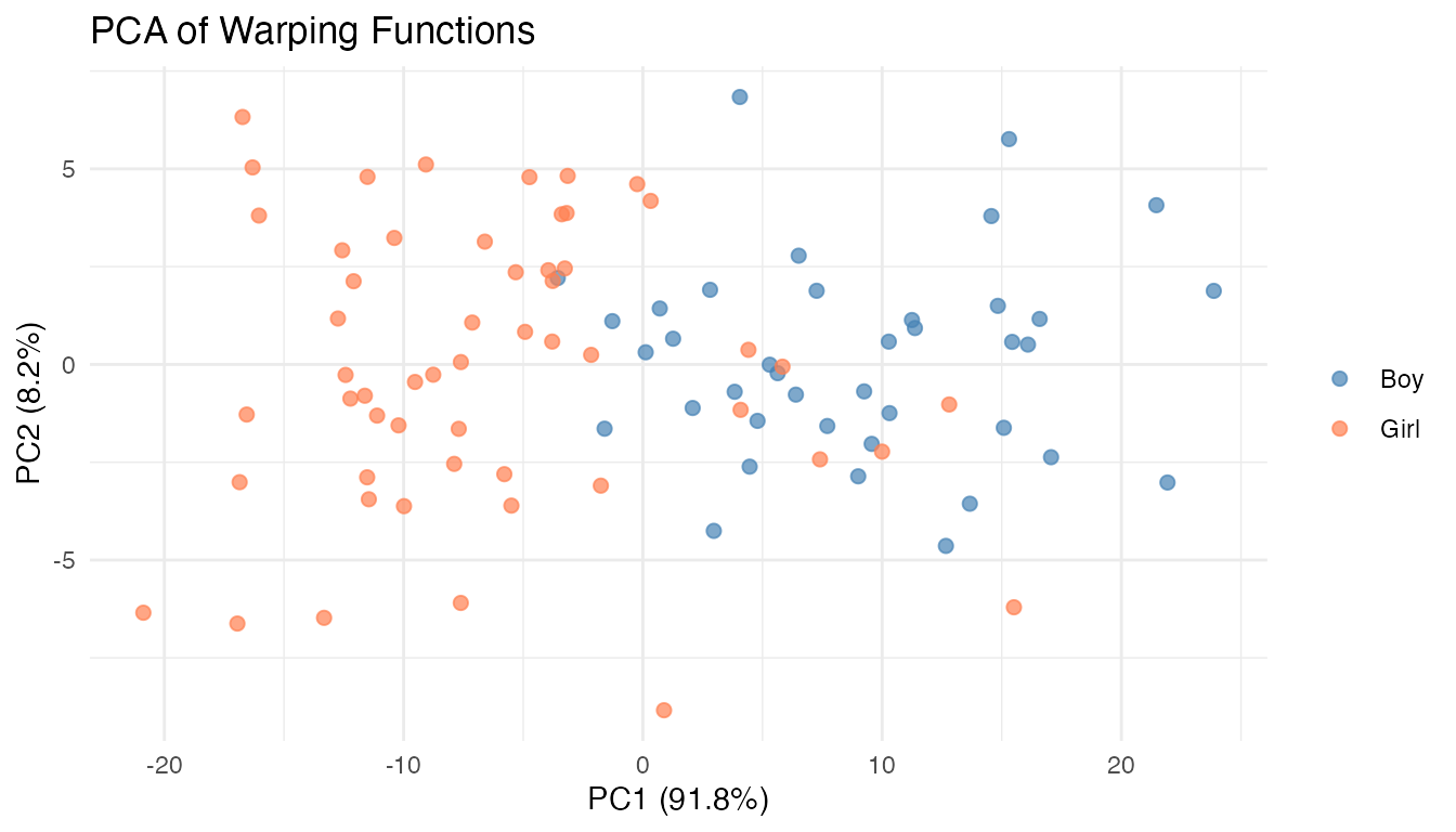
The PC1 score is almost perfectly correlated with the mean timing shift () and clearly separates boys from girls. PC2 captures a secondary mode of timing variation orthogonal to the early/late shift – its interpretation would require inspecting the eigenfunctions.
References
- Tucker, J.D., Wu, W., and Srivastava, A. (2013). Generative models for functional data using phase and amplitude separation. Computational Statistics & Data Analysis, 61:50–66.
- Srivastava, A. and Klassen, E. (2016). Functional and Shape Data Analysis. Springer.
- Ramsay, J.O. and Silverman, B.W. (2005). Functional Data Analysis, 2nd ed. Springer.