TSRVF: Linearized Elastic Analysis

Introduction

After elastic alignment, the aligned curves live on a nonlinear manifold – the quotient space $\mathcal{F} / \Gamma$ of functions modulo reparameterization. Standard linear operations (PCA, regression, hypothesis testing) are not directly valid on this curved space.

The Transported Square-Root Velocity Function (TSRVF) solves this by mapping aligned curves to a tangent space at the Karcher mean, where the geometry is locally Euclidean. In this tangent space, standard multivariate methods apply directly, giving a rigorous framework for elastic functional data analysis.

library(fdars)
#> 
#> Attaching package: 'fdars'
#> The following objects are masked from 'package:stats':
#> 
#>     cov, decompose, deriv, median, sd, var
#> The following object is masked from 'package:base':
#> 
#>     norm
library(ggplot2)
library(patchwork)
theme_set(theme_minimal())

How It Works (Intuition)

After elastic alignment, curve shapes live on a curved surface (a manifold) – think of points on the surface of a globe. Standard statistical methods like PCA assume data lives in a flat space (like a map), so applying them directly to aligned curves introduces distortion.

The TSRVF solves this by projecting curves onto a flat tangent plane at the mean shape – like laying a flat map tangent to the globe at one point. Near the point of contact, the map is a good approximation of the globe’s surface.

Each curve becomes a tangent vector – a direction and magnitude showing how that curve’s shape differs from the mean. These tangent vectors live in ordinary Euclidean space, so you can:

Run PCA to find the main modes of shape variation
Use regression with tangent vectors as predictors
Apply any clustering or classification method that works with vectors

The projection is invertible: you can go from tangent vectors back to curves (by “projecting back onto the globe”), so you can reconstruct curves from their PC scores or model predictions.

Mathematical Framework

The Shape Space

Let $\mathcal{F}$ denote the space of absolutely continuous functions $f : [0, 1] \to \mathbb{R}$ , and let $\Gamma$ be the warping group of orientation-preserving diffeomorphisms of $[0, 1]$ . The shape space is the quotient:

$\mathcal{S} = \mathcal{F} / \Gamma$

where two functions $f_1, f_2$ are equivalent if $f_1 = f_2 \circ \gamma$ for some $\gamma \in \Gamma$ . Points in $\mathcal{S}$ represent curve shapes, stripped of parameterization effects.

Via the SRSF transform $q(t) = \text{sign}(f'(t)) \sqrt{|f'(t)|}$ , the shape space is isometric to the quotient of the unit Hilbert sphere $\mathbb{S}^\infty \subset L^2$ by $\Gamma$ . This is a nonlinear manifold with nontrivial curvature.

Exponential and Logarithmic Maps

At a point $[\mu]$ on the shape space (represented by the Karcher mean), the tangent space $T_{[\mu]} \mathcal{S}$ is a flat (Euclidean) vector space. The exponential map $\exp_{[\mu]}$ projects from the tangent space onto the manifold, and the logarithmic map $\log_{[\mu]}$ does the reverse:

$v_i = \log_{[\mu]}([f_i]) \in T_{[\mu]} \mathcal{S}$

These tangent vectors $v_i$ are the TSRVF representation. They capture how each curve’s shape differs from the mean, in a coordinate system where Euclidean distances approximate geodesic distances on the manifold.

The TSRVF Transform

Given aligned SRSFs $\tilde{q}_i = (q_i \circ \gamma_i^*) \sqrt{\dot\gamma_i^*}$ and the mean SRSF $\bar{q}$ (the Karcher mean in SRSF space), the TSRVF of the $i$ -th curve is computed via the inverse exponential map on the sphere:

$v_i = \frac{\theta_i}{\sin(\theta_i)} \left( \tilde{q}_i - \cos(\theta_i) \, \bar{q} \right)$

where $\theta_i = \cos^{-1}(\langle \tilde{q}_i, \bar{q} \rangle_{L^2})$ is the geodesic distance between $\tilde{q}_i$ and $\bar{q}$ on the sphere.

Key properties:

$v_i \in T_{\bar{q}} \mathbb{S}^\infty$ : the tangent vectors are orthogonal to $\bar{q}$ , i.e., $\langle v_i, \bar{q} \rangle = 0$
Euclidean distances approximate geodesic distances: $\|v_i - v_j\|_{L^2} \approx d_e(f_i, f_j)$ for curves near the mean
Linear operations are valid: addition, scalar multiplication, inner products in the tangent space have geometric meaning

Inverse Transform

To reconstruct a curve from its tangent vector $v$ , we apply the exponential map:

$\tilde{q} = \cos(\|v\|) \, \bar{q} + \sin(\|v\|) \, \frac{v}{\|v\|}$

This gives the aligned SRSF, from which the aligned curve is recovered via SRSF inversion.

Quick Start

set.seed(42)
argvals <- seq(0, 1, length.out = 100)

# Simulate curves with amplitude and phase variation
n <- 20
data <- matrix(0, n, 100)
for (i in 1:n) {
  amp <- rnorm(1, 1, 0.2)
  shift <- runif(1, -0.08, 0.08)
  data[i, ] <- amp * sin(2 * pi * (argvals - shift)) +
               0.3 * rnorm(1) * cos(4 * pi * argvals)
}
fd <- fdata(data, argvals = argvals)

# Compute TSRVF
tv <- tsrvf.transform(fd, max.iter = 15, tol = 1e-4)
print(tv)
#> TSRVF (Transported SRSF)
#>   Curves: 20 x 100 grid points
#>   Converged: TRUE

p1 <- plot(fd) + labs(title = "Original Curves")
p2 <- plot(tv, type = "tangent") + labs(title = "TSRVF Tangent Vectors")
p3 <- plot(tv, type = "mean")
p1 + p2 + p3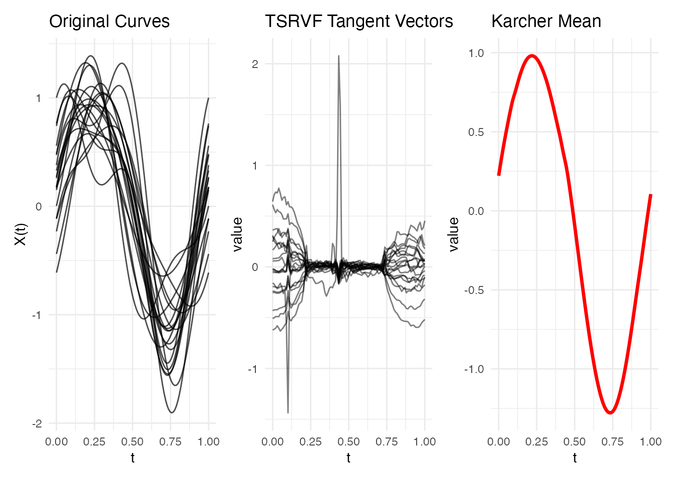

The tangent vectors represent each curve’s shape deviation from the mean in a Euclidean space – ready for PCA, regression, or any linear method.

From a Pre-Computed Alignment

If you have already computed a Karcher mean (which is the expensive step), you can obtain the TSRVF without re-running the alignment:

km <- karcher.mean(fd, max.iter = 15)
tv_from <- tsrvf.from.alignment(km)

# Same tangent space, no extra alignment cost
cat("Dimensions:", nrow(tv_from$tangent_vectors$data), "x",
    ncol(tv_from$tangent_vectors$data), "\n")
#> Dimensions: 20 x 100

Inverse Transform

The TSRVF is invertible – you can reconstruct (aligned) curves from their tangent vectors:

recon <- tsrvf.inverse(tv)

# Compare original aligned curves to reconstruction
p1 <- plot(km, type = "aligned") + labs(title = "Aligned Curves")
p2 <- plot(recon) + labs(title = "Reconstructed from TSRVF")
p1 + p2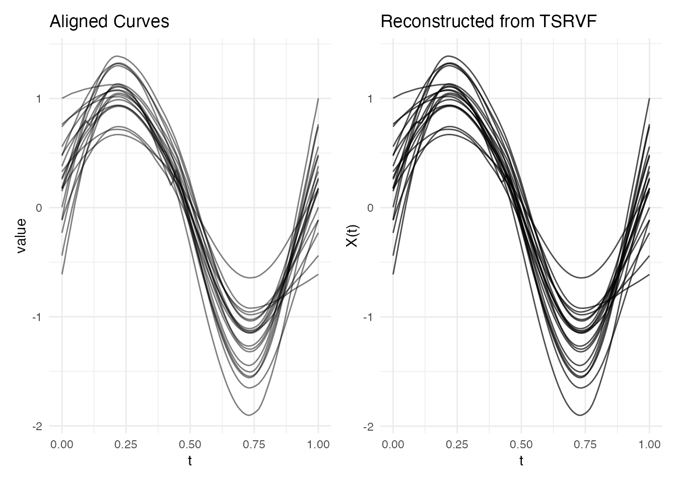

TSRVF-Based PCA

The main application of TSRVF is enabling standard PCA in the tangent space. This gives elastic FPCA – principal components that respect the geometry of the shape space.

# Standard PCA on tangent vectors
tv_data <- tv$tangent_vectors$data
pca_result <- prcomp(tv_data, center = TRUE, scale. = FALSE)

# Variance explained
var_explained <- pca_result$sdev^2 / sum(pca_result$sdev^2)
cat("Variance explained by first 3 PCs:",
    round(cumsum(var_explained)[1:3] * 100, 1), "%\n")
#> Variance explained by first 3 PCs: 83.2 93.8 97.5 %

scores <- pca_result$x[, 1:2]
df_scores <- data.frame(PC1 = scores[, 1], PC2 = scores[, 2])

ggplot(df_scores, aes(x = PC1, y = PC2)) +
  geom_point(size = 2) +
  labs(title = "TSRVF PCA Scores", x = "PC1", y = "PC2") +
  coord_equal()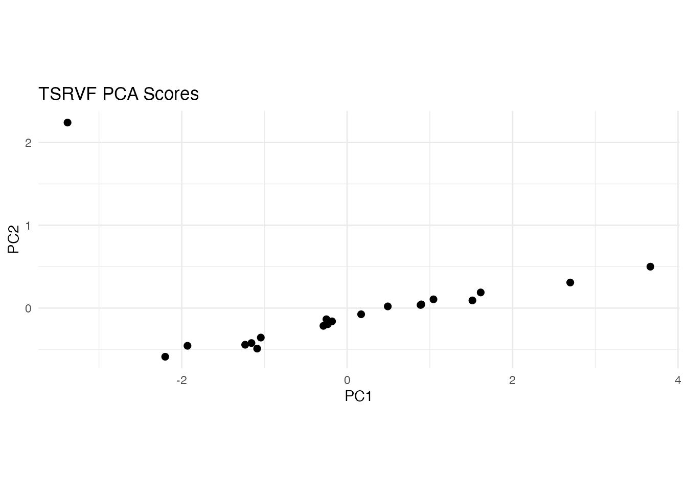

Comparison: Raw FPCA vs TSRVF FPCA

Standard FPCA on the raw (unaligned) data confounds amplitude and phase variation. TSRVF FPCA operates on aligned shapes, so the principal components capture only amplitude variation:

# Raw FPCA
raw_pca <- prcomp(fd$data, center = TRUE, scale. = FALSE)
raw_var <- raw_pca$sdev^2 / sum(raw_pca$sdev^2)

# TSRVF FPCA
tsrvf_var <- var_explained

df_var <- data.frame(
  PC = rep(1:5, 2),
  Variance = c(cumsum(raw_var[1:5]), cumsum(tsrvf_var[1:5])) * 100,
  Method = rep(c("Raw FPCA", "TSRVF FPCA"), each = 5)
)

ggplot(df_var, aes(x = PC, y = Variance, color = Method)) +
  geom_line(linewidth = 1) +
  geom_point(size = 2) +
  labs(title = "Cumulative Variance Explained",
       x = "Number of PCs", y = "Cumulative % Variance") +
  scale_color_manual(values = c("Raw FPCA" = "grey50", "TSRVF FPCA" = "steelblue"))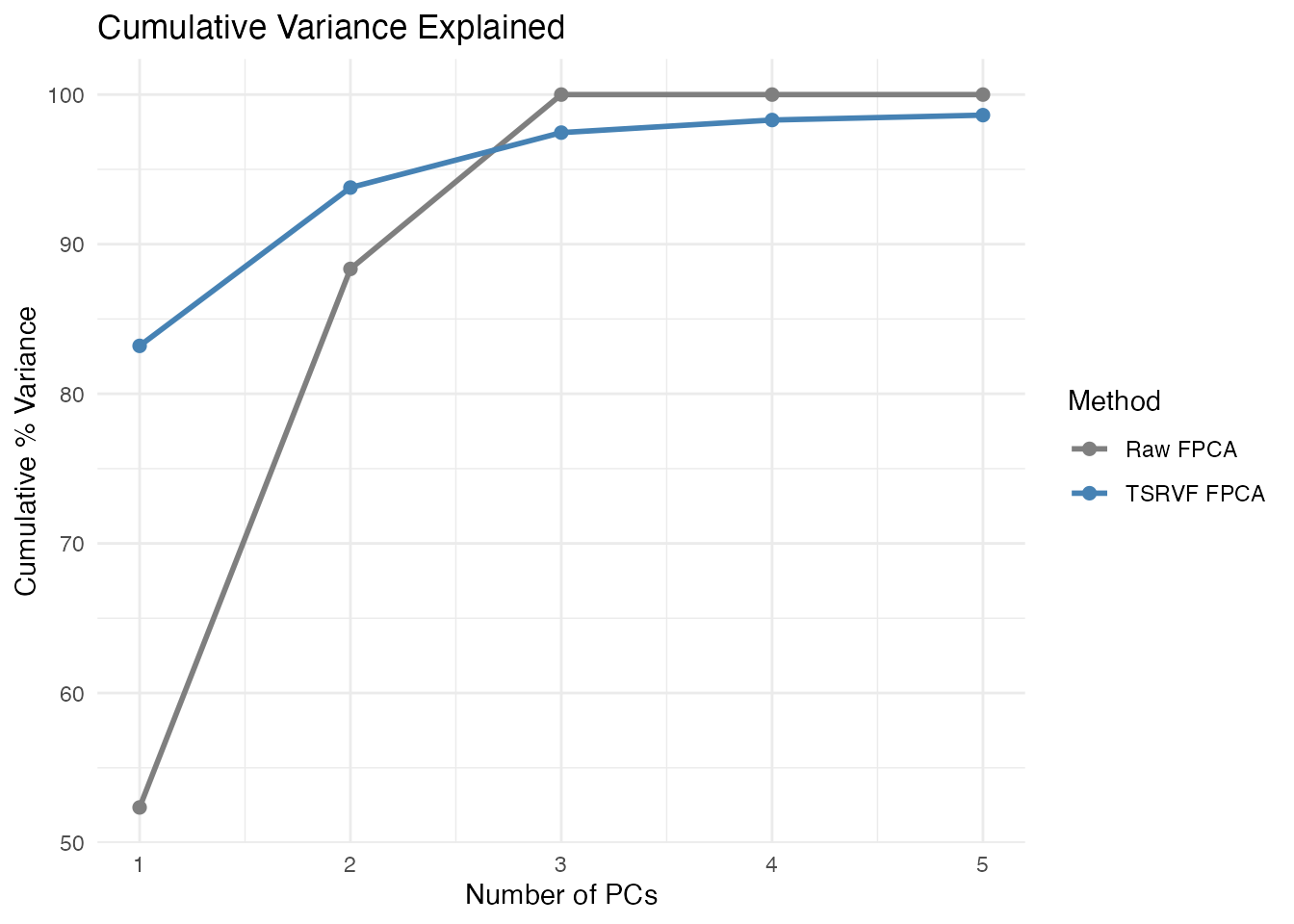

TSRVF FPCA typically needs fewer components because it has already removed phase variation – the remaining amplitude variation is lower-dimensional.

When to Use TSRVF

Scenario	Recommended approach
Exploratory alignment & visualization	`karcher.mean()` / `elastic.align()`
PCA on aligned data	`tsrvf.transform()` + `prcomp()`
Regression with aligned predictors	`tsrvf.transform()` + standard regression
Clustering aligned curves	`tsrvf.transform()` + any Euclidean clustering
Classification	TSRVF scores as features

The key insight: TSRVF converts a nonlinear shape analysis problem into a standard multivariate statistics problem, at the cost of a one-time alignment step.

Introduction

How It Works (Intuition)

Mathematical Framework

The Shape Space

Exponential and Logarithmic Maps

The TSRVF Transform

Inverse Transform

Quick Start

From a Pre-Computed Alignment

Inverse Transform

TSRVF-Based PCA

Comparison: Raw FPCA vs TSRVF FPCA

When to Use TSRVF

See Also