Uncertainty Quantification

Overview

Point predictions alone are insufficient for critical applications. fdars provides four complementary approaches to uncertainty quantification for functional regression models:

Method	Question	Assumptions	Current Models	Function
Prediction Intervals	How uncertain is $\hat{y}$ ?	Gaussian errors	lm only	`fregre.prediction.interval()`
Conformal Prediction	How uncertain is $\hat{y}$ ?	None (distribution-free)	lm, np, elastic, logistic	`conformal.fregre.lm()`, `cv.conformal.regression()`, etc.
LOO Cross-Validation	How well does the model generalise?	None	lm only	`fregre.loo()`
Bootstrap CI for $\beta(t)$	Where is the coefficient significant?	None (bootstrap)	lm + logistic	`fregre.bootstrap.ci()`

Supported Models

Most methods currently require a fregre.lm model (fitted by fregre.lm()). fregre.bootstrap.ci() also supports functional.logistic models.

Prediction intervals and LOO-CV require the hat matrix $\boldsymbol{H}$ , residual standard error $\hat{\sigma}$ , and the FPC score matrix $\boldsymbol{\Xi}$ — internal structures only fregre.lm provides. Nonparametric models like fregre.np() do not produce a hat matrix or parametric variance estimate, so the formulas for prediction intervals and LOO-CV (which exploit $e_i^{(-i)} = e_i / (1 - h_{ii})$ ) do not apply.

Conformal prediction is different. The algorithm is inherently model-agnostic — it only needs a fit/predict function and a set of calibration residuals. The coverage guarantee $P(y_{\text{new}} \in C_\alpha) \geq 1 - \alpha$ holds for any model, with no distributional assumptions. fdars provides conformal inference for linear (fregre.lm), nonparametric (fregre.np), elastic regression, elastic PCR, and logistic models, via split, cross-validation (CV+), jackknife+, and generic conformal interfaces. See Advanced Conformal Methods for details.

Setup

n <- 80
m <- 100
t_grid <- seq(0, 1, length.out = m)

beta_true <- 2 * dnorm(t_grid, 0.3, 0.08) - 1.5 * dnorm(t_grid, 0.7, 0.08)
beta_true <- beta_true / max(abs(beta_true))

X <- matrix(0, n, m)
for (i in 1:n) {
  X[i, ] <- sin(2 * pi * t_grid) + 0.5 * rnorm(1) * cos(4 * pi * t_grid) +
            rnorm(m, sd = 0.1)
}

dt <- t_grid[2] - t_grid[1]
y <- numeric(n)
for (i in 1:n) {
  y[i] <- sum(beta_true * X[i, ]) * dt + rnorm(1, sd = 0.3)
}

fdataobj <- fdata(X, argvals = t_grid)
model <- fregre.lm(fdataobj, y, ncomp = 5)

Prediction-Level Uncertainty

Both methods answer the same question — how uncertain is $\hat{y}$ for a new observation? — but differ in assumptions and interval shape.

Parametric Prediction Intervals

Requires fregre.lm.

In plain English. A prediction interval is like an error bar around each prediction. It says: “the true value will fall in this range with 95% confidence.” Observations that look unusual compared to the training data get wider intervals — the model is less sure about them.

Mathematically. For a new observation with FPC scores $\boldsymbol{\xi}_{\text{new}}$ , the prediction interval accounts for both estimation uncertainty and irreducible noise:

$\hat{y}_{\text{new}} \pm t_{n-K-1,\,1-\alpha/2}\;\hat{\sigma}\sqrt{1 + \boldsymbol{\xi}_{\text{new}}^\top (\boldsymbol{\Xi}^\top\boldsymbol{\Xi})^{-1} \boldsymbol{\xi}_{\text{new}}}.$

The term $\boldsymbol{\xi}_{\text{new}}^\top (\boldsymbol{\Xi}^\top\boldsymbol{\Xi})^{-1} \boldsymbol{\xi}_{\text{new}}$ is the leverage — how far the new point is from the training centre in FPC score space. High leverage observations receive wider intervals.

pred_int <- fregre.prediction.interval(
  model,
  train.data = fdataobj,
  new.data = fdataobj[1:20],
  confidence = 0.95
)

df_pi <- data.frame(
  Observation = 1:20,
  Observed = y[1:20],
  Fitted = pred_int$predictions,
  Lower = pred_int$lower,
  Upper = pred_int$upper
)

ggplot(df_pi, aes(x = .data$Observation)) +
  geom_ribbon(aes(ymin = .data$Lower, ymax = .data$Upper),
              fill = "#4A90D9", alpha = 0.2) +
  geom_point(aes(y = .data$Observed), color = "#D55E00", size = 2) +
  geom_line(aes(y = .data$Fitted), color = "#4A90D9", linewidth = 1) +
  labs(title = "95% Prediction Intervals",
       subtitle = "Blue band = prediction interval, red points = observed values",
       x = "Observation", y = "y")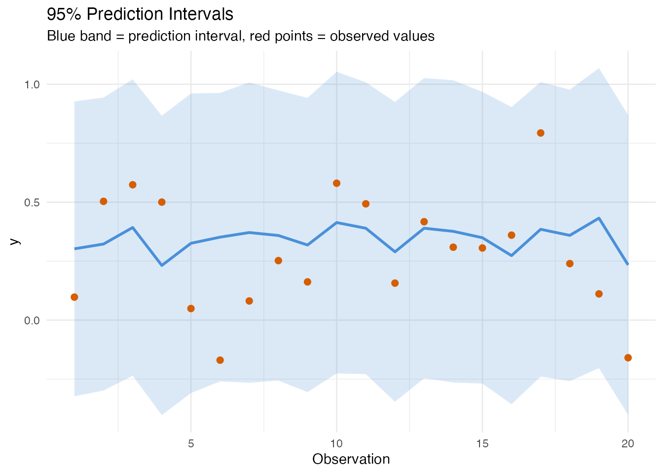

Coverage and Width

covered <- df_pi$Observed >= df_pi$Lower & df_pi$Observed <= df_pi$Upper
cat("Coverage:", round(mean(covered) * 100, 1), "%  (expected: 95%)\n")
#> Coverage: 100 %  (expected: 95%)

Wider intervals indicate observations far from the training data centre:

df_pi$Width <- df_pi$Upper - df_pi$Lower

ggplot(df_pi, aes(x = .data$Observation, y = .data$Width)) +
  geom_col(fill = "#7B2D8E", alpha = 0.7) +
  labs(title = "Prediction Interval Widths",
       subtitle = "Wider = more uncertain (high leverage)",
       x = "Observation", y = "Interval Width")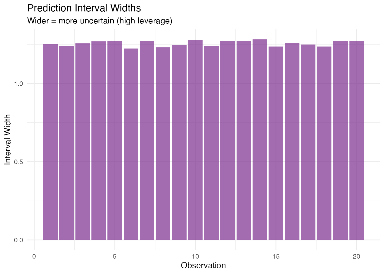

Conformal Prediction

Split conformal is shown here for fregre.lm. See Advanced Conformal Methods below for CV+, jackknife+, nonparametric, and generic conformal variants.

In plain English. Conformal prediction makes no assumptions about the data distribution. Instead of relying on Gaussian theory, it sets aside a portion of the training data as a “calibration set”, measures how wrong the model is on those held-out points, and uses the worst-case error as the interval width. The result: guaranteed coverage (e.g., 90% of future observations will fall in the interval) no matter what the data looks like.

Why is it model-agnostic in theory? The algorithm only needs two things: (1) a fit function that trains a model on data, and (2) a predict function that produces predictions for new data. It computes residuals on the calibration set, takes the $(1-\alpha)$ -quantile, and adds/subtracts that from predictions. No hat matrix, no variance formula, no distributional assumptions.

Mathematically. (Vovk et al., 2005) The split conformal approach provides finite-sample coverage:

$P(y_{\text{new}} \in C_\alpha) \geq 1 - \alpha,$

for any distribution of $(X, y)$ . Given calibration residuals $|e_1|, \ldots, |e_m|$ and quantile $q = \lceil (1 - \alpha)(m + 1) \rceil / m$ -th order statistic, the interval is

$C_\alpha = \left[\hat{y}_{\text{new}} - q,\;\hat{y}_{\text{new}} + q\right].$

All intervals have the same width $2q$ — unlike parametric intervals, which vary with leverage.

# Train/test split
train_fd <- fdataobj[1:60]
train_y <- y[1:60]
test_fd <- fdataobj[61:80]
test_y <- y[61:80]

model_train <- fregre.lm(train_fd, train_y, ncomp = 5)

# Conformal prediction intervals (90% coverage)
conf <- fregre.conformal(
  model_train,
  train.data = train_fd,
  train.y = train_y,
  test.data = test_fd,
  cal.fraction = 0.25,
  alpha = 0.10,
  seed = 42
)

cat("Residual quantile:", round(conf$residual_quantile, 4), "\n")
#> Residual quantile: 0.8114

df_conf <- data.frame(
  Observation = 1:20,
  Observed = test_y,
  Predicted = conf$predictions,
  Lower = conf$lower,
  Upper = conf$upper
)

ggplot(df_conf, aes(x = .data$Observation)) +
  geom_ribbon(aes(ymin = .data$Lower, ymax = .data$Upper),
              fill = "#2E8B57", alpha = 0.2) +
  geom_point(aes(y = .data$Observed), color = "#D55E00", size = 2) +
  geom_line(aes(y = .data$Predicted), color = "#2E8B57", linewidth = 1) +
  labs(title = "90% Conformal Prediction Intervals",
       subtitle = "Green band = conformal interval (distribution-free)",
       x = "Test Observation", y = "y")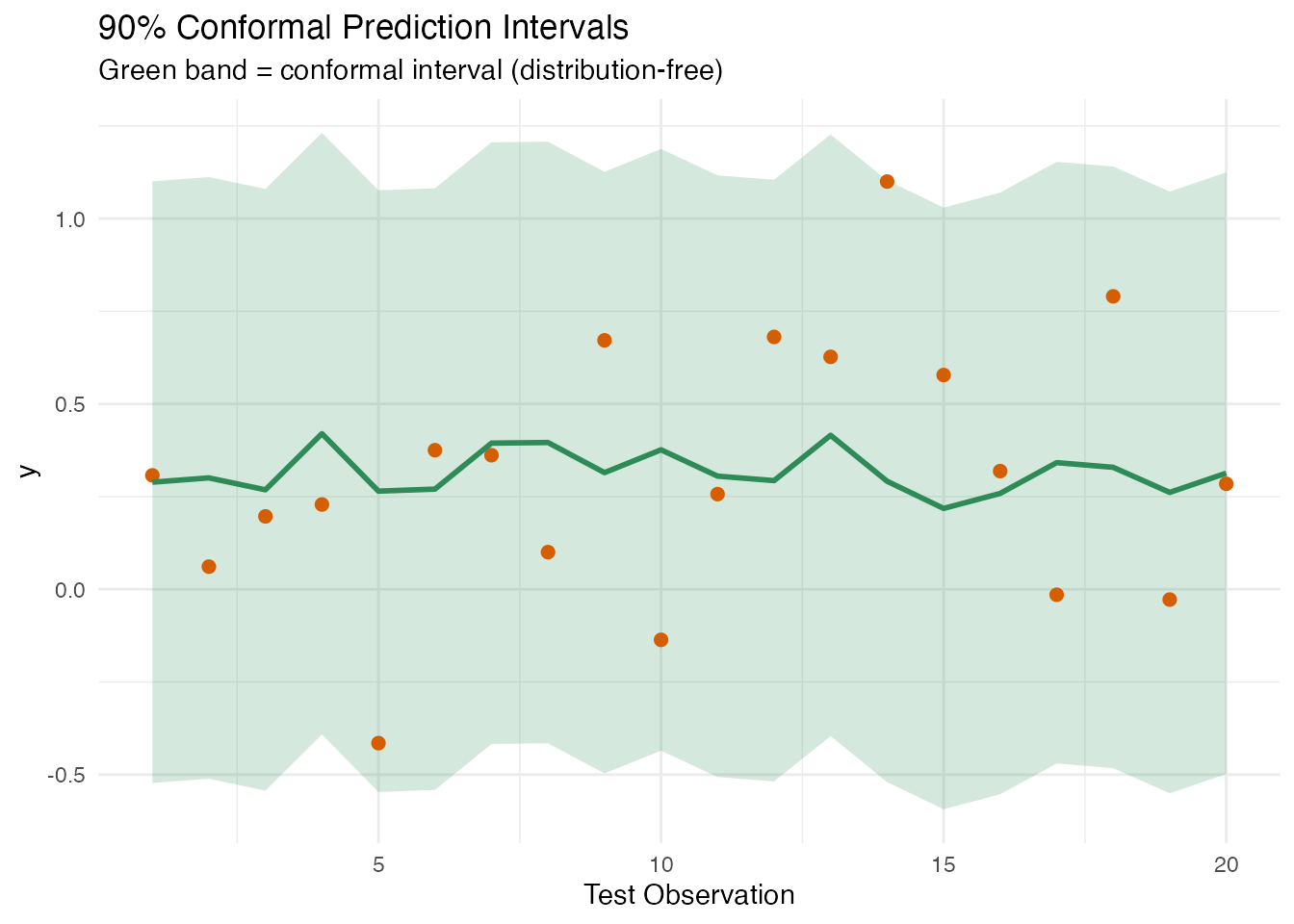

covered_conf <- df_conf$Observed >= df_conf$Lower &
                df_conf$Observed <= df_conf$Upper
cat("Empirical coverage:", round(mean(covered_conf) * 100, 1),
    "%  (target: 90%)\n")
#> Empirical coverage: 100 %  (target: 90%)

Comparison: Parametric vs Conformal

	Parametric	Conformal
Assumptions	Gaussian errors	None
Width	Variable (leverage-dependent)	Constant
Coverage guarantee	Exact if assumptions hold	Finite-sample, always
Data cost	Uses all training data	Sacrifices a calibration fraction
Model support	`fregre.lm` only	Any model (in theory)

pred_param <- fregre.prediction.interval(
  model_train, train.data = train_fd, new.data = test_fd, confidence = 0.90
)

df_compare <- data.frame(
  Method = rep(c("Parametric", "Conformal"), each = 20),
  Width = c(pred_param$upper - pred_param$lower,
            conf$upper - conf$lower)
)

ggplot(df_compare, aes(x = .data$Method, y = .data$Width, fill = .data$Method)) +
  geom_boxplot(alpha = 0.7) +
  scale_fill_manual(values = c("Parametric" = "#4A90D9",
                               "Conformal" = "#2E8B57")) +
  labs(title = "Interval Width: Parametric vs Conformal",
       subtitle = "Both at 90% nominal level",
       y = "Interval Width") +
  theme(legend.position = "none")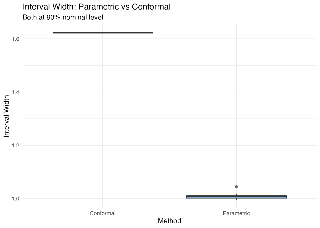

Model Assessment: LOO Cross-Validation

Requires fregre.lm.

In plain English. Leave-one-out cross-validation asks: “If I re-fit the model without observation $i$ , how well does it predict that observation?” Doing this for every observation gives an honest estimate of how the model will perform on new data. A large gap between in-sample $R^2$ and LOO $R^2$ signals overfitting — the model has memorised the training data.

The clever part: for linear models, you don’t actually need to re-fit $n$ times. The hat matrix gives you the answer in one step.

Mathematically. The LOO residual for observation $i$ is efficiently computed via the hat matrix:

$e_{i}^{(-i)} = \frac{e_i}{1 - h_{ii}},$

where $h_{ii}$ is the $i$ -th diagonal of $\boldsymbol{H} = \boldsymbol{\Xi}(\boldsymbol{\Xi}^\top\boldsymbol{\Xi})^{-1}\boldsymbol{\Xi}^\top$ . High-leverage points ( $h_{ii}$ close to 1) have inflated LOO residuals — removing them changes the fit substantially.

The PRESS statistic is

$\text{PRESS} = \sum_{i=1}^{n} \left(e_i^{(-i)}\right)^2,$

and the LOO $R^2 = 1 - \text{PRESS} / \text{TSS}$ provides an honest estimate of out-of-sample performance.

loo <- fregre.loo(model, data = fdataobj, y = y)

cat("PRESS:", round(loo$press, 4), "\n")
#> PRESS: 7.8572
cat("LOO R\u00b2:", round(loo$loo_r_squared, 4), "\n")
#> LOO R²: -0.0757
cat("In-sample R\u00b2:", round(model$r.squared, 4), "\n")
#> In-sample R²: 0.0607

A large gap between in-sample $R^2$ and LOO $R^2$ indicates overfitting.

df_loo <- data.frame(
  Observation = seq_along(loo$loo_residuals),
  LOO_Residual = loo$loo_residuals,
  In_Sample_Residual = model$residuals
)

ggplot(df_loo, aes(x = .data$In_Sample_Residual, y = .data$LOO_Residual)) +
  geom_point(color = "#7B2D8E", size = 2, alpha = 0.7) +
  geom_abline(slope = 1, intercept = 0, linetype = "dashed",
              color = "gray50") +
  labs(title = "In-Sample vs LOO-CV Residuals",
       subtitle = "Points above the diagonal indicate optimistic in-sample fit",
       x = "In-sample Residual", y = "LOO Residual")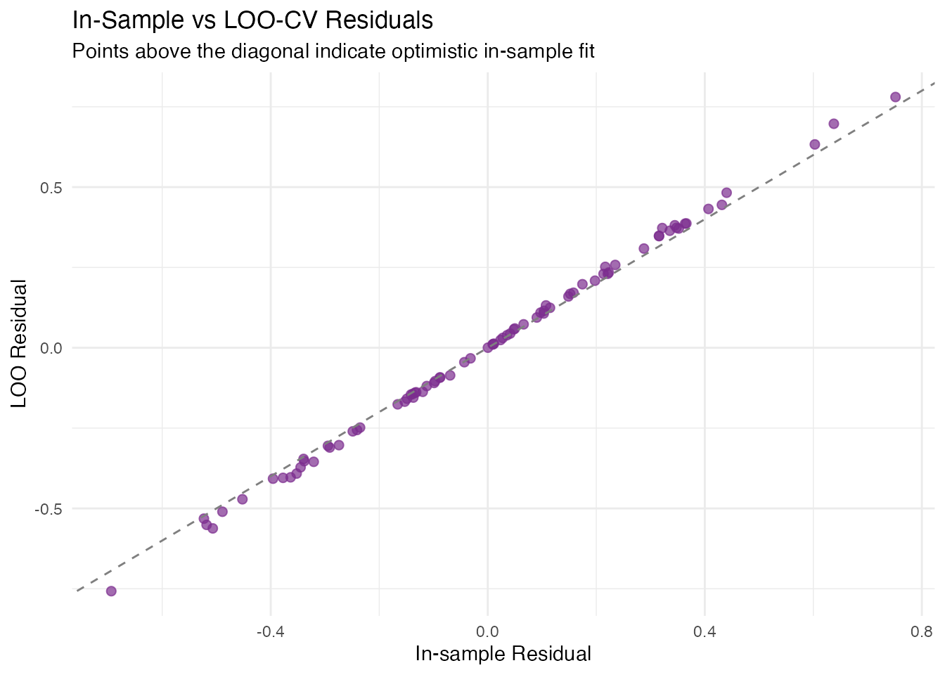

df_leverage <- data.frame(
  Observation = seq_along(loo$loo_residuals),
  LOO_Residual = abs(loo$loo_residuals),
  In_Sample_Residual = abs(model$residuals)
)
df_leverage$Inflation <- df_leverage$LOO_Residual / df_leverage$In_Sample_Residual

ggplot(df_leverage, aes(x = .data$Observation, y = .data$Inflation)) +
  geom_col(fill = "#7B2D8E", alpha = 0.6) +
  geom_hline(yintercept = 1, linetype = "dashed", color = "gray50") +
  labs(title = "LOO Residual Inflation Factor",
       subtitle = "|LOO residual| / |in-sample residual| — high values = high leverage",
       x = "Observation", y = "Inflation (1 / (1 − h_ii))")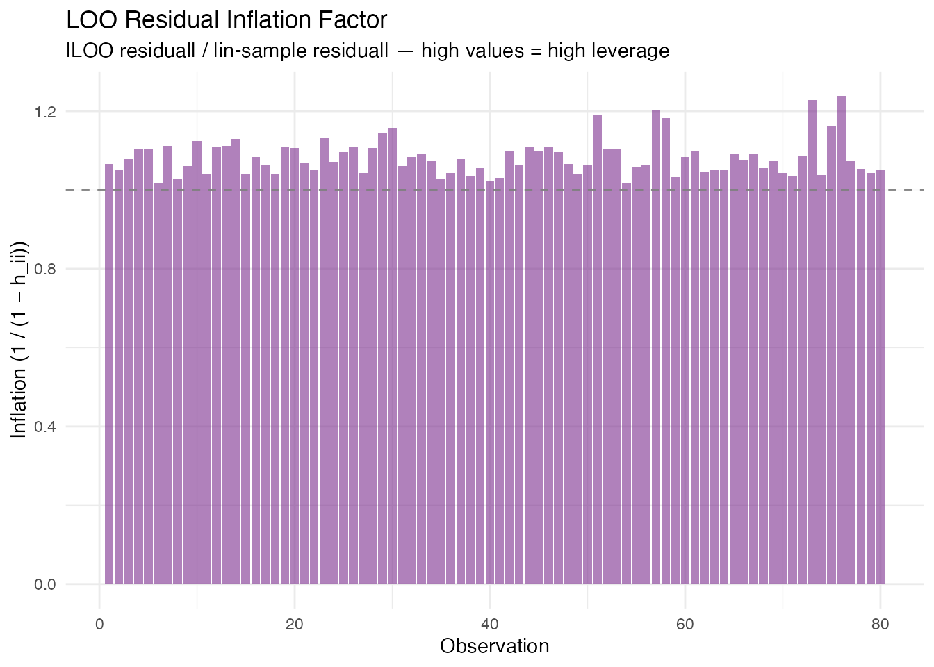

Coefficient Uncertainty: Bootstrap CI for β(t)

Supports both fregre.lm and functional.logistic.

Bootstrap CI: pointwise vs simultaneous bands

In plain English. Previous sections quantified uncertainty in predictions ( $\hat{y}$ ). This section asks a different question: where on the functional domain does the predictor actually matter? The functional coefficient $\beta(t)$ tells you how each part of the curve contributes to the response. Bootstrap confidence bands show which parts of $\beta(t)$ are reliably different from zero — those are the regions where the predictor has a statistically significant effect.

The bootstrap works by resampling the data many times, fitting the model each time, and observing how $\hat{\beta}(t)$ varies. If it varies a lot at some $t$ , we’re uncertain about that part of the coefficient.

Mathematically. Given $B$ bootstrap replicates $\hat{\beta}^{*1}(t), \ldots, \hat{\beta}^{*B}(t)$ , we construct two types of confidence bands:

Pointwise Bands

At each grid point $t$ independently:

$CI_{\text{pw}}(t) = \left[\hat{\beta}_{(\alpha/2)}^*(t),\;\hat{\beta}_{(1-\alpha/2)}^*(t)\right],$

where $\hat{\beta}_{(q)}^*(t)$ is the $q$ -quantile of the bootstrap distribution at $t$ . This controls coverage at each $t$ separately but not simultaneously across all $t$ .

ci <- fregre.bootstrap.ci(model, n.boot = 200, alpha = 0.05, seed = 42)
print(ci)
#> Bootstrap Confidence Intervals for beta(t)
#>   Model type: fregre.lm 
#>   Alpha: 0.05 
#>   Bootstrap replicates: 200 / 200 succeeded
#>   Grid points: 100

plot(ci)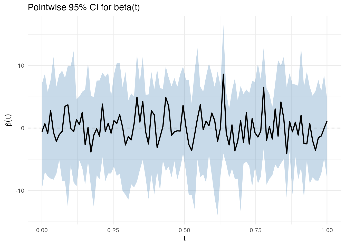

Simultaneous Bands

In plain English. Pointwise bands control the error at each grid point separately. If you have 100 grid points and test each at 5%, you’d expect about 5 false positives. Simultaneous bands are wider — they guarantee that the entire curve $\beta(t)$ lies within the band with $(1-\alpha)$ probability. Regions where the simultaneous band excludes zero are statistically significant at the chosen level, corrected for the multiple testing across all $t$ .

Mathematically. The simultaneous band uses the sup-norm critical value $c_\alpha$ estimated from the bootstrap distribution:

$CI_{\text{sim}}(t) = \hat{\beta}(t) \pm c_\alpha \cdot \widehat{SE}_{\text{boot}}(t),$

where $c_\alpha$ is the $(1-\alpha)$ -quantile of $\sup_t |\hat{\beta}^*(t) - \hat{\beta}(t)| / \widehat{SE}_{\text{boot}}(t)$ over the bootstrap replicates.

plot(ci, simultaneous = TRUE)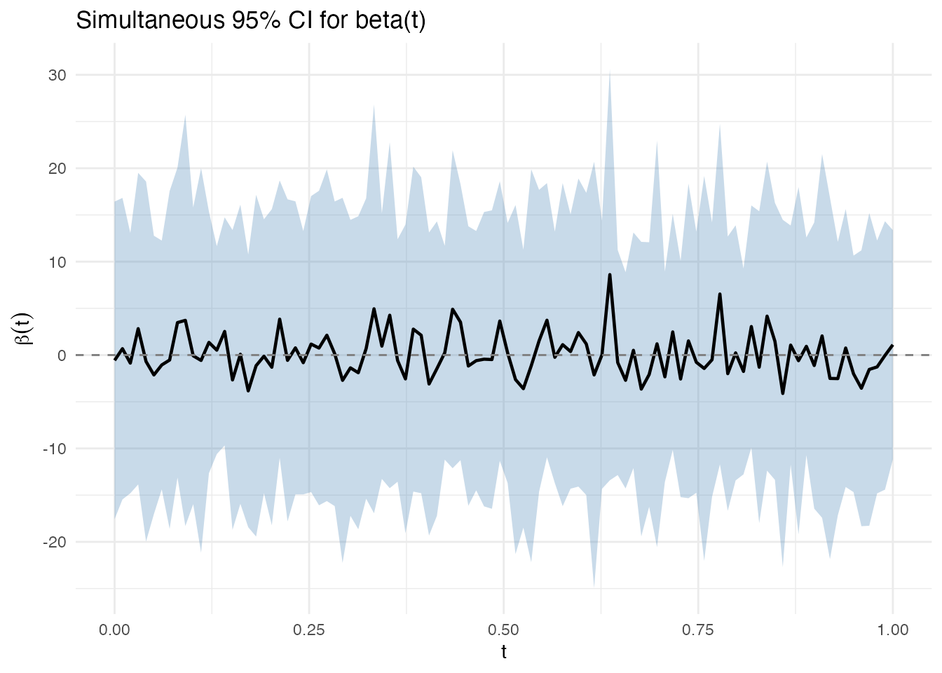

The simultaneous band is wider because it guarantees $P(\beta(t) \in CI_{\text{sim}}(t) \;\forall\, t) \geq 1 - \alpha$ , rather than controlling coverage at each $t$ separately.

Advanced Conformal Methods

The split conformal method above uses a single calibration/training split. fdars also provides cross-conformal (CV+) and jackknife+ variants that use all data for both training and calibration, typically producing tighter intervals.

Cross-Conformal (CV+) Regression

CV+ conformal: K-fold calibration with no data waste

CV+ conformal runs K-fold cross-validation internally: each fold serves as the calibration set for the model trained on the remaining folds. This avoids the data-splitting penalty of split conformal — all observations contribute to both training and calibration.

The coverage guarantee is slightly weaker than split conformal ( $1 - 2\alpha$ in theory), but empirically CV+ intervals are tighter with near-nominal coverage.

# CV+ conformal with fregre.lm (5-fold)
cv_conf <- cv.conformal.regression(
  train_fd, train_y, test_fd,
  method = "fregre.lm",
  ncomp = 5, n.folds = 5,
  alpha = 0.10, seed = 42
)

cat("CV+ coverage:", round(cv_conf$coverage * 100, 1), "%\n")
#> CV+ coverage: 91.7 %
cat("CV+ mean width:", round(mean(cv_conf$upper - cv_conf$lower), 4), "\n")
#> CV+ mean width: 0.9646

CV+ also works with the nonparametric model fregre.np, which has no parametric prediction intervals — conformal is the only rigorous UQ method available:

cv_conf_np <- cv.conformal.regression(
  train_fd, train_y, test_fd,
  method = "fregre.np",
  ncomp = 5, n.folds = 5,
  alpha = 0.10, seed = 42
)

cat("CV+ (nonparametric) coverage:", round(cv_conf_np$coverage * 100, 1), "%\n")
#> CV+ (nonparametric) coverage: 91.7 %

Jackknife+ Regression

Jackknife+ is the leave-one-out analogue: each training observation is left out once, the model is fitted on the remaining $n-1$ observations, and the left-out residual calibrates the interval. This is the most data-efficient conformal method but requires $n$ model fits.

jk <- jackknife.plus(
  train_fd, train_y, test_fd,
  method = "fregre.lm",
  ncomp = 5, alpha = 0.10
)

cat("Jackknife+ coverage:", round(jk$coverage * 100, 1), "%\n")
#> Jackknife+ coverage: 91.7 %
cat("Jackknife+ mean width:", round(mean(jk$upper - jk$lower), 4), "\n")
#> Jackknife+ mean width: 1.0765

Generic Conformal from a Fitted Model

Generic conformal: post-hoc UQ from a fitted model

If you already have a fitted fregre.lm model, conformal.generic.regression() constructs conformal intervals without re-fitting. It uses the model’s FPCA components to split and calibrate internally:

gen_conf <- conformal.generic.regression(
  model_train, train_fd, train_y, test_fd,
  cal.fraction = 0.25, alpha = 0.10, seed = 42
)
#> Warning: conformal.generic.regression uses the pre-fitted model without
#> refitting. Calibration residuals are in-sample, so coverage guarantee is
#> broken. Supply calibration.indices (held-out indices) for valid coverage, or
#> use conformal.fregre.lm() / cv.conformal.regression() instead.

cat("Generic conformal coverage:", round(gen_conf$coverage * 100, 1), "%\n")
#> Generic conformal coverage: 100 %

Comparing All Conformal Variants

Conformal methods at a glance: split, CV+, jackknife+, generic

df_all <- data.frame(
  Method = rep(c("Split", "CV+", "Jackknife+", "Generic"), each = length(test_y)),
  Width = c(
    conf$upper - conf$lower,
    cv_conf$upper - cv_conf$lower,
    jk$upper - jk$lower,
    gen_conf$upper - gen_conf$lower
  )
)

ggplot(df_all, aes(x = .data$Method, y = .data$Width, fill = .data$Method)) +
  geom_boxplot(alpha = 0.7) +
  scale_fill_manual(values = c("Split" = "#2E8B57", "CV+" = "#4A90D9",
                                "Jackknife+" = "#D55E00", "Generic" = "#7B2D8E")) +
  labs(title = "Interval Width by Conformal Method",
       subtitle = "All at 90% nominal level",
       y = "Interval Width") +
  theme(legend.position = "none")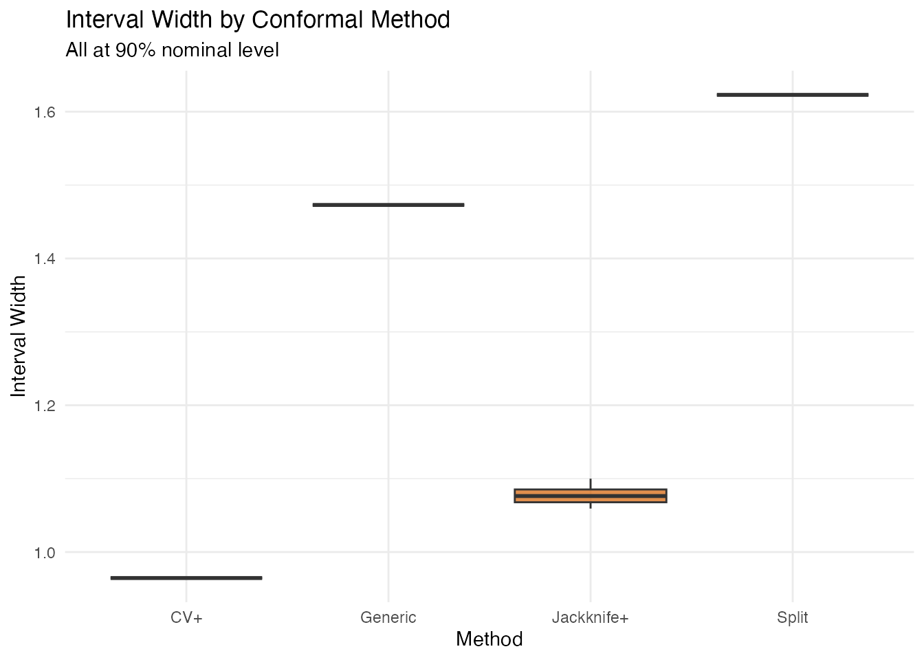

Variant	Function	Data use	# model fits	Guarantee
Split	`conformal.fregre.lm()`	Wastes calibration data	1	$\geq 1 - \alpha$
CV+	`cv.conformal.regression()`	All data used	$K$	$\geq 1 - 2\alpha$
Jackknife+	`jackknife.plus()`	All data used	$n$	$\geq 1 - 2\alpha$
Generic	`conformal.generic.regression()`	From fitted model	0 (pre-fitted)	Heuristic only $^*$

$^*$ Generic conformal uses in-sample calibration residuals (model trained on all data). Coverage guarantee is broken. Use split or CV+ for valid coverage.

Summary

Aspect	Prediction Intervals	Conformal	LOO-CV	Bootstrap CI
Target	$\hat{y}$	$\hat{y}$	Model fit	$\beta(t)$
Models	lm only	lm, np, elastic, logistic	lm only	lm + logistic
Assumptions	Gaussian	None	None	None
Width	Variable (leverage)	Constant (split) or variable (CV+)	—	Variable (SE)
Guarantee	Exact if Gaussian	Finite-sample	—	Asymptotic
Key output	Interval bounds	Interval bounds	PRESS, LOO $R^2$	Pointwise + simultaneous bands

References

Allen, D.M. (1974). The relationship between variable selection and data augmentation and a method for prediction. Technometrics, 16(1), 125–127.
Ramsay, J.O. and Silverman, B.W. (2005). Functional Data Analysis. 2nd ed. Springer.
Vovk, V., Gammerman, A. and Shafer, G. (2005). Algorithmic Learning in a Random World. Springer.
Barber, R.F., Candes, E.J., Ramdas, A. and Tibshirani, R.J. (2021). Predictive inference with the jackknife+. Annals of Statistics, 49(1), 486–507.
Romano, Y., Patterson, E. and Candes, E. (2019). Conformalized quantile regression. Advances in Neural Information Processing Systems, 32.