Distance Metrics and Semimetrics

Introduction

Distance measures are fundamental to many FDA methods including clustering, k-nearest neighbors regression, and outlier detection. fdars provides both true metrics (satisfying the triangle inequality) and semimetrics (which may not).

Choosing the right distance measure depends on what kind of “similarity” matters for your application. Some distances compare curves point-by-point (L2), others allow for timing shifts before comparing (DTW, Soft-DTW, elastic), and still others focus on specific aspects like curve shape (derivative-based) or frequency content (Fourier-based).

A metric $d$ on a space $\mathcal{X}$ satisfies:

1. $d(f, g) \geq 0$ (non-negativity)
2. $d(f, g) = 0 \Leftrightarrow f = g$ (identity of indiscernibles)
3. $d(f, g) = d(g, f)$ (symmetry)
4. $d(f, h) \leq d(f, g) + d(g, h)$ (triangle inequality)

A semimetric satisfies only conditions 1-3.

library(fdars)
#> 
#> Attaching package: 'fdars'
#> The following objects are masked from 'package:stats':
#> 
#>     cov, decompose, deriv, median, sd, var
#> The following object is masked from 'package:base':
#> 
#>     norm
library(ggplot2)
theme_set(theme_minimal())

# Create example data with different curve types
set.seed(42)
m <- 100
t_grid <- seq(0, 1, length.out = m)

# Four types of curves
curve1 <- sin(2 * pi * t_grid)                    # Sine
curve2 <- sin(2 * pi * t_grid + 0.5)              # Phase-shifted sine
curve3 <- cos(2 * pi * t_grid)                    # Cosine
curve4 <- sin(4 * pi * t_grid)                    # Higher frequency

X <- rbind(curve1, curve2, curve3, curve4)
fd <- fdata(X, argvals = t_grid,
            names = list(main = "Four Curve Types"))
plot(fd)

True Metrics

Lp Distance (metric.lp)

The $L^p$ distance is the most common choice for functional data. It computes the integrated $L^p$ norm of the difference between two functions:

$$d_p(f, g) = \left( \int_{\mathcal{T}} |f(t) - g(t)|^p \, dt \right)^{1/p}$$

For discrete observations, this is approximated using numerical integration (Simpson’s rule):

$$d_p(f, g) \approx \left( \sum_{j=1}^{m} w_j |f(t_j) - g(t_j)|^p \right)^{1/p}$$

where $w_j$ are quadrature weights.

Special cases:

• $p = 2$ (L2/Euclidean): Most common, corresponds to the standard functional norm. Sensitive to vertical differences.
• $p = 1$ (L1/Manhattan): More robust to outliers than L2.
• $p = \infty$ (L-infinity/Chebyshev): Maximum absolute difference, $d_\infty(f, g) = \max_t |f(t) - g(t)|$.

# L2 (Euclidean) distance - default
dist_l2 <- metric.lp(fd)
print(round(as.matrix(dist_l2), 3))
#>        curve1 curve2 curve3 curve4
#> curve1   0.00  0.350  1.000      1
#> curve2   0.35  0.000  0.722      1
#> curve3   1.00  0.722  0.000      1
#> curve4   1.00  1.000  1.000      0

# L1 (Manhattan) distance
dist_l1 <- metric.lp(fd, lp = 1)

# L-infinity (maximum) distance
dist_linf <- metric.lp(fd, lp = Inf)

Weighted Lp Distance

Apply different weights to different parts of the domain:

$$d_{p,w}(f, g) = \left( \int_{\mathcal{T}} w(t) |f(t) - g(t)|^p \, dt \right)^{1/p}$$

This is useful when certain parts of the domain are more important than others.

# Weight emphasizing the middle of the domain
w <- dnorm(t_grid, mean = 0.5, sd = 0.2)
w <- w / sum(w) * length(w)  # Normalize

dist_weighted <- metric.lp(fd, lp = 2, w = w)

Hausdorff Distance (metric.hausdorff)

The Hausdorff distance treats curves as sets of points $(t, f(t))$ in 2D space and computes the maximum of minimum distances:

$$d_H(f, g) = \max\left\{ \sup_{t \in \mathcal{T}} \inf_{s \in \mathcal{T}} \|P_f(t) - P_g(s)\|, \sup_{s \in \mathcal{T}} \inf_{t \in \mathcal{T}} \|P_f(t) - P_g(s)\| \right\}$$

where $P_f(t) = (t, f(t))$ is the point on the graph of $f$ at time $t$.

The Hausdorff distance is useful when:

• Curves may cross each other
• The timing of features is less important than their shape
• Comparing curves with different supports

dist_haus <- metric.hausdorff(fd)
print(round(as.matrix(dist_haus), 3))
#>        curve1 curve2 curve3 curve4
#> curve1  0.000  0.479  0.678  0.328
#> curve2  0.479  0.000  0.521  0.416
#> curve3  0.678  0.521  0.000  0.352
#> curve4  0.328  0.416  0.352  0.000

Dynamic Time Warping (metric.DTW)

DTW allows for non-linear alignment of curves before computing the distance. It finds the optimal warping path $\pi$ that minimizes:

$$d_{DTW}(f, g) = \min_{\pi} \sqrt{\sum_{(i,j) \in \pi} |f(t_i) - g(t_j)|^2}$$

subject to boundary conditions, monotonicity, and continuity constraints.

The Sakoe-Chiba band constraint limits the warping to $|i - j| \leq w$, preventing excessive distortion:

$$d_{DTW}^{SC}(f, g) = \min_{\pi: |i-j| \leq w} \sqrt{\sum_{(i,j) \in \pi} |f(t_i) - g(t_j)|^2}$$

DTW is particularly effective for:

• Phase-shifted signals
• Time series with varying speed
• Comparing signals with local time distortions

dist_dtw <- metric.DTW(fd)
print(round(as.matrix(dist_dtw), 3))
#>        curve1 curve2 curve3 curve4
#> curve1  0.000  1.452 18.185 24.844
#> curve2  1.452  0.000  3.488 25.980
#> curve3 18.185  3.488  0.000 40.825
#> curve4 24.844 25.980 40.825  0.000

Notice that DTW gives a smaller distance between the original sine and phase-shifted sine compared to L2, because it can align them:

# Compare L2 vs DTW for phase-shifted curves
cat("L2 distance (sine vs phase-shifted):", round(as.matrix(dist_l2)[1, 2], 3), "\n")
#> L2 distance (sine vs phase-shifted): 0.35
cat("DTW distance (sine vs phase-shifted):", round(as.matrix(dist_dtw)[1, 2], 3), "\n")
#> DTW distance (sine vs phase-shifted): 1.452

DTW with band constraint:

# Restrict warping to 10% of the series length
dist_dtw_band <- metric.DTW(fd, w = round(m * 0.1))

Soft-DTW (metric.softDTW)

Soft-DTW (Cuturi & Blondel, 2017) is a differentiable relaxation of DTW that replaces the hard minimum with a soft minimum controlled by a smoothing parameter $\gamma > 0$:

$$\text{sdtw}_\gamma(f, g) = \min_\gamma^{\text{soft}} \sum_{(i,j) \in \pi} |f(t_i) - g(t_j)|^2$$

where $\min^\text{soft}$ is the log-sum-exp soft minimum: $\min^\text{soft}(a_1, \ldots, a_n) = -\gamma \log \sum_k \exp(-a_k / \gamma)$.

As $\gamma \to 0$, Soft-DTW converges to standard DTW. As $\gamma \to \infty$, all warping paths receive equal weight. Soft-DTW is not a metric – it can assign negative values to self-distances. The Soft-DTW divergence corrects this:

$$D_\gamma(f, g) = \text{sdtw}_\gamma(f, g) - \frac{1}{2}\left[ \text{sdtw}_\gamma(f, f) + \text{sdtw}_\gamma(g, g) \right]$$

The divergence is non-negative, zero iff $f = g$, and symmetric.

# Soft-DTW distance matrix (raw)
dist_sdtw <- metric.softDTW(fd, gamma = 1.0)
cat("Soft-DTW distance matrix:\n")
#> Soft-DTW distance matrix:
print(round(as.matrix(dist_sdtw), 3))
#>          curve1   curve2   curve3   curve4
#> curve1    0.000 -162.953 -126.778 -104.031
#> curve2 -162.953    0.000 -152.837 -103.278
#> curve3 -126.778 -152.837    0.000  -80.142
#> curve4 -104.031 -103.278  -80.142    0.000

# Soft-DTW divergence (non-negative, symmetric)
dist_sdtw_div <- metric.softDTW(fd, gamma = 1.0, divergence = TRUE)
cat("\nSoft-DTW divergence matrix:\n")
#> 
#> Soft-DTW divergence matrix:
print(round(as.matrix(dist_sdtw_div), 3))
#>        curve1 curve2 curve3 curve4
#> curve1  0.000  5.635 41.658 62.441
#> curve2  5.635  0.000 15.562 63.158
#> curve3 41.658 15.562  0.000 86.142
#> curve4 62.441 63.158 86.142  0.000

Effect of the Smoothing Parameter $\gamma$

Small $\gamma$ approximates hard DTW (sharper, less smooth gradients); large $\gamma$ averages over more warping paths (smoother, less discriminative):

gammas <- c(0.01, 0.1, 1.0, 10.0)
sdtw_12 <- sapply(gammas, function(g) {
  as.matrix(metric.softDTW(fd, gamma = g, divergence = TRUE))[1, 2]
})

df_gamma <- data.frame(gamma = gammas, divergence = sdtw_12)
ggplot(df_gamma, aes(x = gamma, y = divergence)) +
  geom_line(linewidth = 1) +
  geom_point(size = 2) +
  scale_x_log10() +
  labs(title = "Soft-DTW Divergence vs Smoothing Parameter",
       subtitle = "Distance between sine and phase-shifted sine",
       x = expression(gamma ~ "(log scale)"), y = "Divergence")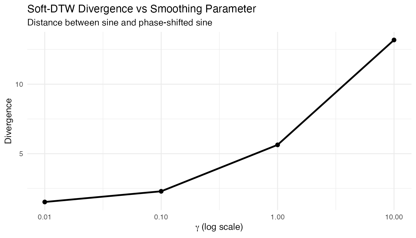

Soft-DTW Barycenter

Soft-DTW provides a differentiable loss, making it suitable for computing barycenters (weighted averages under DTW alignment) via gradient descent:

# Create shifted bumps for barycenter computation
set.seed(42)
n_bary <- 10
X_bary <- matrix(0, n_bary, m)
for (i in 1:n_bary) {
  shift <- runif(1, -0.1, 0.1)
  X_bary[i, ] <- exp(-80 * (t_grid - 0.5 - shift)^2)
}
fd_bary <- fdata(X_bary, argvals = t_grid)

bc <- softdtw.barycenter(fd_bary, gamma = 1.0)
cross_mean <- colMeans(fd_bary$data)

df_bc <- data.frame(
  t = rep(t_grid, 2),
  value = c(as.numeric(bc$barycenter$data), cross_mean),
  type = rep(c("Soft-DTW Barycenter", "Cross-sectional Mean"), each = m)
)

ggplot() +
  geom_line(data = data.frame(
    t = rep(t_grid, n_bary),
    value = as.vector(t(fd_bary$data)),
    curve = rep(1:n_bary, each = m)
  ), aes(x = t, y = value, group = curve), alpha = 0.25) +
  geom_line(data = df_bc, aes(x = t, y = value, color = type), linewidth = 1.2) +
  scale_color_manual(values = c("Cross-sectional Mean" = "steelblue",
                                 "Soft-DTW Barycenter" = "firebrick")) +
  labs(title = "Soft-DTW Barycenter vs Cross-Sectional Mean",
       x = "t", y = "f(t)", color = NULL)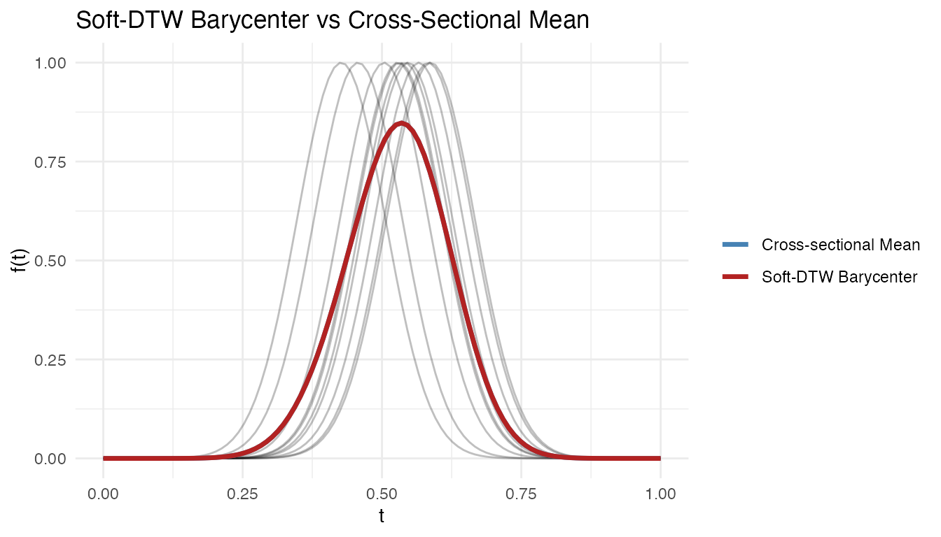

The cross-sectional mean is attenuated by the phase shifts; the Soft-DTW barycenter recovers the peak shape by accounting for alignment.

Kullback-Leibler Divergence (metric.kl)

The symmetric Kullback-Leibler divergence treats normalized curves as probability density functions:

$$d_{KL}(f, g) = \frac{1}{2}\left[ \int f(t) \log\frac{f(t)}{g(t)} \, dt + \int g(t) \log\frac{g(t)}{f(t)} \, dt \right]$$

Before computing, curves are shifted to be non-negative and normalized to integrate to 1:

$$\tilde{f}(t) = \frac{f(t) - \min_s f(s) + \epsilon}{\int [f(s) - \min_s f(s) + \epsilon] \, ds}$$

This metric is useful for:

• Comparing density-like functions
• Distribution comparison
• Information-theoretic analysis

# Shift curves to be positive for KL
X_pos <- X - min(X) + 0.1
fd_pos <- fdata(X_pos, argvals = t_grid)

dist_kl <- metric.kl(fd_pos)
print(round(as.matrix(dist_kl), 3))
#>        curve1 curve2 curve3 curve4
#> curve1  0.000  0.139  1.208  1.187
#> curve2  0.139  0.000  0.630  1.426
#> curve3  1.208  0.630  0.000  1.156
#> curve4  1.187  1.426  1.156  0.000

Semimetrics

Semimetrics may not satisfy the triangle inequality but can be more appropriate for certain applications or provide computational advantages.

PCA-Based Semimetric (semimetric.pca)

Projects curves onto the first $q$ principal components and computes the Euclidean distance in the reduced space:

$$d_{PCA}(f, g) = \sqrt{\sum_{k=1}^{q} (\xi_k^f - \xi_k^g)^2}$$

where $\xi_k^f = \langle f - \bar{f}, \phi_k \rangle$ is the $k$-th principal component score of $f$, and $\phi_k$ are the eigenfunctions from functional PCA.

This semimetric is useful for:

• Dimension reduction before distance computation
• Noise reduction (low-rank approximation)
• Computational efficiency with many evaluation points

# Distance using first 3 PCs
dist_pca <- semimetric.pca(fd, ncomp = 3)
print(round(as.matrix(dist_pca), 3))
#>        [,1]  [,2]   [,3]   [,4]
#> [1,]  0.000 3.514 10.000  9.950
#> [2,]  3.514 0.000  7.198  9.961
#> [3,] 10.000 7.198  0.000 10.000
#> [4,]  9.950 9.961 10.000  0.000

Derivative-Based Semimetric (semimetric.deriv)

Computes the $L^p$ distance based on the $r$-th derivative of the curves:

$$d_{deriv}^{(r)}(f, g) = \left( \int_{\mathcal{T}} |f^{(r)}(t) - g^{(r)}(t)|^p \, dt \right)^{1/p}$$

where $f^{(r)}$ denotes the $r$-th derivative of $f$.

This semimetric focuses on the shape and dynamics of curves rather than their absolute values. It is particularly useful when:

• Comparing rate of change (first derivative)
• Analyzing curvature (second derivative)
• Functions are measured with different baselines

# First derivative (velocity)
dist_deriv1 <- semimetric.deriv(fd, nderiv = 1)

# Second derivative (acceleration/curvature)
dist_deriv2 <- semimetric.deriv(fd, nderiv = 2)

cat("First derivative distances:\n")
#> First derivative distances:
print(round(as.matrix(dist_deriv1), 3))
#>       [,1]  [,2]  [,3]  [,4]
#> [1,] 0.000 2.197 6.279 9.912
#> [2,] 2.197 0.000 4.530 9.912
#> [3,] 6.279 4.530 0.000 9.912
#> [4,] 9.912 9.912 9.912 0.000

Basis Semimetric (semimetric.basis)

Projects curves onto a basis (B-spline or Fourier) and computes the Euclidean distance between the coefficient vectors:

$$d_{basis}(f, g) = \|c^f - c^g\|_2 = \sqrt{\sum_{k=1}^{K} (c_k^f - c_k^g)^2}$$

where $c^f = (c_1^f, \ldots, c_K^f)$ are the basis coefficients from $f(t) \approx \sum_{k=1}^{K} c_k^f B_k(t)$.

For B-splines: Local support provides good approximation of local features.

For Fourier basis: Global support captures periodic patterns efficiently.

# B-spline basis (local features)
dist_bspline <- semimetric.basis(fd, nbasis = 15, basis = "bspline")

# Fourier basis (periodic patterns)
dist_fourier <- semimetric.basis(fd, nbasis = 11, basis = "fourier")

cat("B-spline basis distances:\n")
#> B-spline basis distances:
print(round(as.matrix(dist_bspline), 3))
#>       [,1]  [,2]  [,3]  [,4]
#> [1,] 0.000 1.509 4.015 3.913
#> [2,] 1.509 0.000 2.771 3.999
#> [3,] 4.015 2.771 0.000 4.289
#> [4,] 3.913 3.999 4.289 0.000

Fourier Semimetric (semimetric.fourier)

Uses the Fast Fourier Transform (FFT) to compute Fourier coefficients and measures distance based on the first $K$ frequency components:

$$d_{FFT}(f, g) = \sqrt{\sum_{k=0}^{K} |\hat{f}_k - \hat{g}_k|^2}$$

where $\hat{f}_k$ is the $k$-th Fourier coefficient computed via FFT.

This is computationally efficient for large datasets and particularly useful for periodic or frequency-domain analysis.

dist_fft <- semimetric.fourier(fd, nfreq = 5)
cat("Fourier (FFT) distances:\n")
#> Fourier (FFT) distances:
print(round(as.matrix(dist_fft), 3))
#>        curve1 curve2 curve3 curve4
#> curve1  0.000  0.005  0.012  0.694
#> curve2  0.005  0.000  0.008  0.695
#> curve3  0.012  0.008  0.000  0.700
#> curve4  0.694  0.695  0.700  0.000

Horizontal Shift Semimetric (semimetric.hshift)

Finds the optimal horizontal shift before computing the $L^2$ distance:

$$d_{hshift}(f, g) = \min_{|h| \leq h_{max}} \left( \int_{\mathcal{T}} |f(t) - g(t+h)|^2 \, dt \right)^{1/2}$$

where $h$ is the shift in discrete time units and $h_{max}$ is the maximum allowed shift.

This semimetric is simpler than DTW (only horizontal shifts, no warping) but can be very effective for:

• Phase-shifted periodic signals
• ECG or other physiological signals with timing variations
• Comparing curves where horizontal alignment is meaningful

dist_hshift <- semimetric.hshift(fd)
cat("Horizontal shift distances:\n")
#> Horizontal shift distances:
print(round(as.matrix(dist_hshift), 3))
#>        curve1 curve2 curve3 curve4
#> curve1  0.000  0.005  0.010  0.733
#> curve2  0.005  0.000  0.005  0.629
#> curve3  0.010  0.005  0.000  0.718
#> curve4  0.733  0.629  0.718  0.000

Elastic Distances

Elastic alignment provides a family of distances based on the Fisher-Rao metric and the SRSF transform. These distances decompose curve differences into amplitude (shape) and phase (timing) components. See vignette("elastic-alignment", package = "fdars") for the full framework.

Elastic Distance (metric.elastic / elastic.distance)

The elastic distance computes the $L^2$ distance between optimally aligned SRSFs:

$$d_e(f, g) = \min_{\gamma \in \Gamma} \| q_f - (q_g \circ \gamma) \sqrt{\dot\gamma} \|_{L^2}$$

where $q_f, q_g$ are the SRSFs of $f, g$ and $\Gamma$ is the warping group. This is a proper metric that is invariant to reparameterization.

dist_elastic <- elastic.distance(fd)
cat("Elastic distance matrix:\n")
#> Elastic distance matrix:
print(round(dist_elastic, 3))
#>       [,1]  [,2]  [,3]  [,4]
#> [1,] 0.000 0.354 1.212 1.950
#> [2,] 0.354 0.000 0.841 1.954
#> [3,] 1.212 0.841 0.000 2.130
#> [4,] 1.950 1.954 2.130 0.000

Amplitude Distance (amplitude.distance)

The amplitude distance measures the shape difference between curves after optimal alignment – it captures how much the curves differ in height, depth, and feature magnitude:

$$d_a(f_1, f_2) = \| q_1 - (q_2 \circ \gamma^*) \sqrt{\dot\gamma^*} \|_{L^2} - \lambda \int_0^1 |\dot\gamma^*(t) - 1| \, dt$$

where $\lambda$ controls the penalty on warping complexity.

dist_amp <- amplitude.distance(fd, lambda = 0)
cat("Amplitude distance matrix:\n")
#> Amplitude distance matrix:
print(round(as.matrix(dist_amp), 3))
#>        curve1 curve2 curve3 curve4
#> curve1  0.000  0.354  1.212  1.950
#> curve2  0.354  0.000  0.841  1.954
#> curve3  1.212  0.841  0.000  2.130
#> curve4  1.950  1.954  2.130  0.000

Phase Distance (phase.distance)

The phase distance measures only the timing difference between curves – how much one curve’s time axis must be warped to match another:

$$d_p(f_1, f_2) = \arccos\left( \int_0^1 \sqrt{\dot\gamma^*(t)} \, dt \right)$$

This is the geodesic distance of the warping function from the identity on the warping group $\Gamma$, which forms a Riemannian manifold.

dist_phase <- phase.distance(fd, lambda = 0)
cat("Phase distance matrix:\n")
#> Phase distance matrix:
print(round(as.matrix(dist_phase), 3))
#>        curve1 curve2 curve3 curve4
#> curve1  0.000  0.119  0.414  0.412
#> curve2  0.119  0.000  0.334  0.414
#> curve3  0.414  0.334  0.000  0.511
#> curve4  0.412  0.414  0.511  0.000

Comparing Amplitude and Phase Distances

The amplitude and phase distances capture orthogonal aspects of curve variability. Curves that differ mainly in timing (phase-shifted copies of the same shape) will have small amplitude distance but large phase distance:

amp_vals <- as.vector(as.matrix(dist_amp))[upper.tri(as.matrix(dist_amp))]
phase_vals <- as.vector(as.matrix(dist_phase))[upper.tri(as.matrix(dist_phase))]

plot(amp_vals, phase_vals, pch = 19, col = "steelblue",
     xlab = "Amplitude Distance", ylab = "Phase Distance",
     main = "Amplitude vs Phase Pairwise Distances")
abline(h = mean(phase_vals), lty = 2, col = "grey50")
abline(v = mean(amp_vals), lty = 2, col = "grey50")

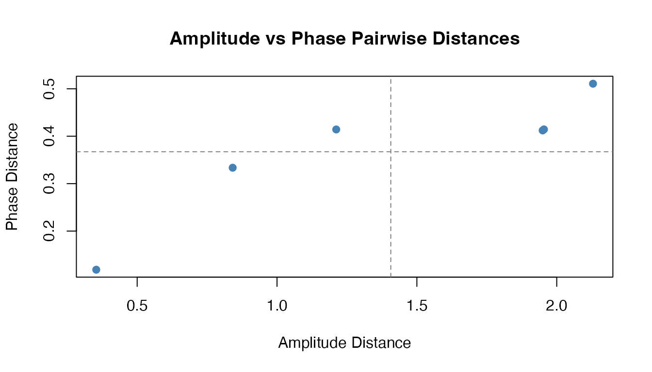
Unified Interface

Use metric() for a unified interface to all distance functions:

# Different methods via single function
d1 <- metric(fd, method = "lp", lp = 2)
d2 <- metric(fd, method = "dtw")
d3 <- metric(fd, method = "hausdorff")
d4 <- metric(fd, method = "pca", ncomp = 2)
d5 <- metric(fd, method = "softdtw", gamma = 1.0)
d6 <- metric(fd, method = "elastic")
d7 <- metric(fd, method = "amplitude")
d8 <- metric(fd, method = "phase")

Comparing Distance Measures

Different distance measures capture different aspects of curve similarity:

# Create comparison data
dists <- list(
  L2 = as.vector(as.matrix(dist_l2)),
  L1 = as.vector(as.matrix(dist_l1)),
  DTW = as.vector(as.matrix(dist_dtw)),
  Hausdorff = as.vector(as.matrix(dist_haus))
)

# Correlation between distance measures
dist_mat <- do.call(cbind, dists)
cat("Correlation between distance measures:\n")
#> Correlation between distance measures:
print(round(cor(dist_mat), 2))
#>             L2   L1  DTW Hausdorff
#> L2        1.00 1.00 0.82      0.74
#> L1        1.00 1.00 0.82      0.74
#> DTW       0.82 0.82 1.00      0.32
#> Hausdorff 0.74 0.74 0.32      1.00

Distance Matrices for Larger Samples

# Generate larger sample
set.seed(123)
n <- 50
X_large <- matrix(0, n, m)
for (i in 1:n) {
  phase <- runif(1, 0, 2*pi)
  freq <- sample(1:3, 1)
  X_large[i, ] <- sin(freq * pi * t_grid + phase) + rnorm(m, sd = 0.1)
}
fd_large <- fdata(X_large, argvals = t_grid)

# Compute distance matrix
dist_matrix <- metric.lp(fd_large)

# Visualize as heatmap using ggplot2
dist_df <- expand.grid(Curve1 = 1:n, Curve2 = 1:n)
dist_df$Distance <- as.vector(as.matrix(dist_matrix))

ggplot(dist_df, aes(x = Curve1, y = Curve2, fill = Distance)) +
  geom_tile() +
  scale_fill_viridis_c(option = "magma") +
  coord_equal() +
  labs(x = "Curve", y = "Curve", title = "L2 Distance Matrix") +
  theme_minimal()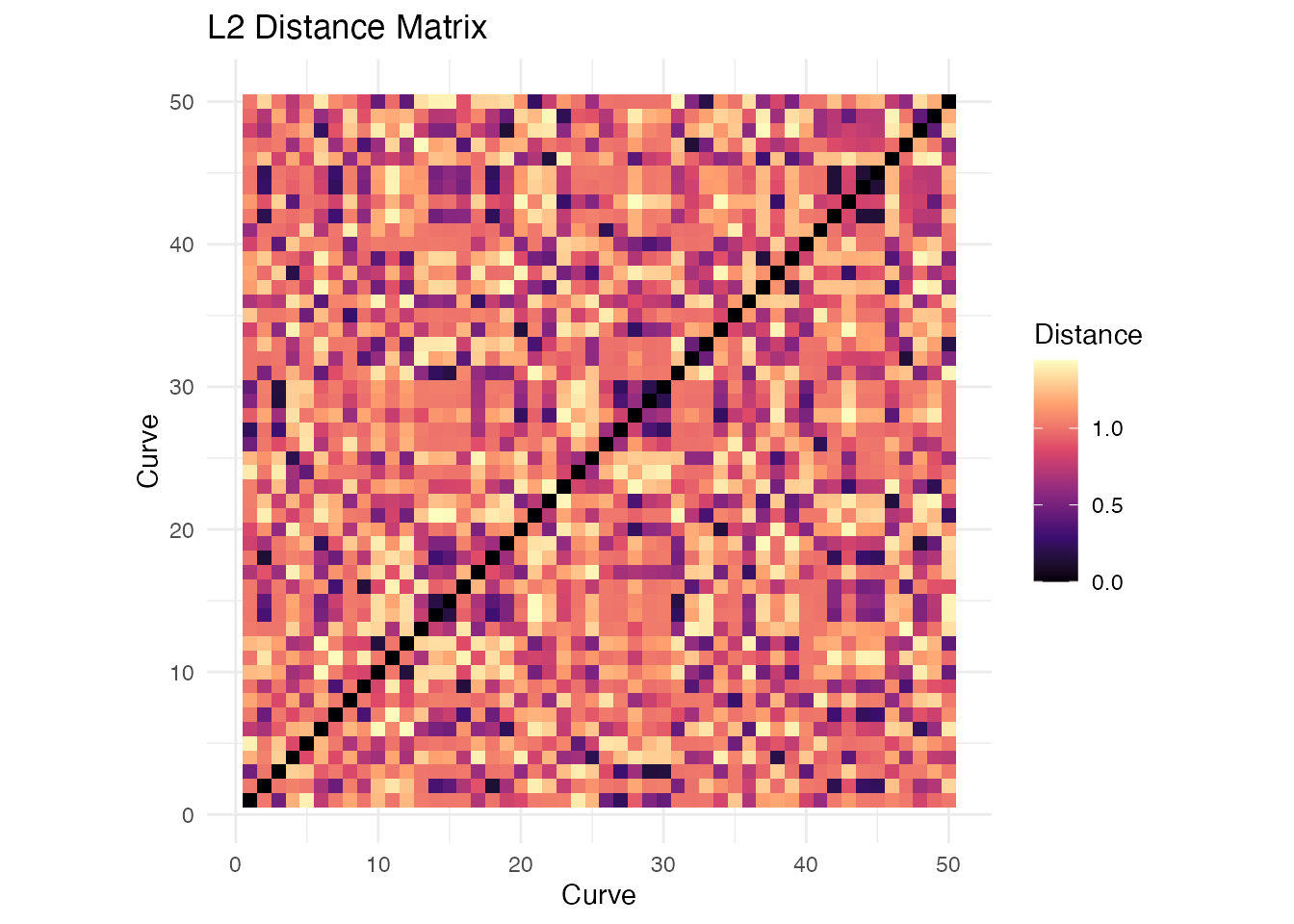

Metric Properties Summary

Distance	Type	Triangle Ineq.	Phase Invariant	Computational Cost
Lp	Metric	Yes	No	O(nm)
Hausdorff	Metric	Yes	Partial	O(nm²)
DTW	Metric*	Yes*	Yes	O(nm²)
Soft-DTW	Semimetric	No	Yes	O(nm²)
Soft-DTW Div.	Semimetric	No***	Yes	O(nm²)
Elastic	Metric	Yes	Yes	O(nm²)
Amplitude	Semimetric	No	Yes	O(nm²)
Phase	Metric	Yes	Yes	O(nm²)
KL	Semimetric	No	No	O(nm)
PCA	Semimetric	Yes**	No	O(nm + nq²)
Derivative	Semimetric	Yes**	No	O(nm)
Basis	Semimetric	Yes**	No	O(nmK)
Fourier	Semimetric	Yes**	No	O(nm log m)
H-shift	Semimetric	No	Yes	O(nm·h_max)

* DTW satisfies triangle inequality when using the same warping path ** These satisfy triangle inequality in the reduced/transformed space *** Soft-DTW divergence is non-negative and symmetric but does not satisfy triangle inequality

Choosing a Distance Measure

Scenario	Recommended Distance
General purpose	L2 (metric.lp)
Heavy-tailed noise	L1 (metric.lp, p=1)
Worst-case analysis	L-infinity (metric.lp, p=Inf)
Phase-shifted signals	DTW, H-shift, or Elastic
Differentiable DTW loss	Soft-DTW (metric.softDTW)
Reparameterization-invariant	Elastic (elastic.distance)
Separate shape vs timing	Amplitude + Phase distances
Curves that cross	Hausdorff
High-dimensional data	PCA-based
Shape comparison	Derivative-based
Periodic data	Fourier-based
Density-like curves	Kullback-Leibler

Performance

Distance computations are parallelized in Rust:

# Benchmark for 500 curves
X_bench <- matrix(rnorm(500 * 200), 500, 200)
fd_bench <- fdata(X_bench)

system.time(metric.lp(fd_bench))
#>    user  system elapsed
#>   0.089   0.000   0.045

system.time(metric.DTW(fd_bench))
#>    user  system elapsed
#>   1.234   0.000   0.312

Using Distances in Other Methods

Distance functions can be passed to clustering and regression:

# K-means with L1 distance
km_l1 <- cluster.kmeans(fd_large, ncl = 3, metric = "L1", seed = 42)

# K-means with custom metric function
km_dtw <- cluster.kmeans(fd_large, ncl = 3, metric = metric.DTW, seed = 42)

# Nonparametric regression uses distances internally
y <- rnorm(n)
fit_np <- fregre.np(fd_large, y, metric = metric.lp)

See Also

• vignette("elastic-alignment", package = "fdars") – elastic alignment framework, Karcher mean, amplitude-phase decomposition
• vignette("alignment-comparison", package = "fdars") – comparing alignment methods side-by-side

References

• Berndt, D.J. and Clifford, J. (1994). Using Dynamic Time Warping to Find Patterns in Time Series. KDD Workshop, 359-370.
• Cuturi, M. and Blondel, M. (2017). Soft-DTW: a Differentiable Loss Function for Time-Series. Proceedings of the 34th International Conference on Machine Learning, 894-903.
• Ferraty, F. and Vieu, P. (2006). Nonparametric Functional Data Analysis. Springer.
• Ramsay, J.O. and Silverman, B.W. (2005). Functional Data Analysis. Springer, 2nd edition.
• Sakoe, H. and Chiba, S. (1978). Dynamic programming algorithm optimization for spoken word recognition. IEEE Transactions on Acoustics, Speech, and Signal Processing, 26(1), 43-49.
• Srivastava, A. and Klassen, E. (2016). Functional and Shape Data Analysis. Springer.