Scalar-on-Function Regression

Introduction

Scalar-on-function regression predicts a scalar response $Y$ from a functional predictor $X(t)$. This is the most common regression setting in functional data analysis: you have curves and want to predict a number.

Which Method Should I Use?

Method	Function	Key parameter	Best when
FPC Regression	fregre.lm()	$K$ (# components)	Default choice; full diagnostics/explainability
PC Regression	fregre.pc()	$K$ (# components)	Pure R alternative to fregre.lm()
Basis Expansion	fregre.basis()	$\lambda$ (penalty)	Smooth $\beta(t)$, interpretable coefficient
Nonparametric	fregre.np()	$h$ (bandwidth) or $k$	Nonlinear relationships
Elastic	elastic.regression()	$\lambda$, warps	Phase-variable curves

Quick decision rule:

1. Start with fregre.lm() — it has the richest downstream support (explainability, diagnostics, uncertainty quantification).
2. Test linearity with flm.test(). If rejected, try fregre.np().
3. If curves are misaligned, consider elastic.regression() (see vignette("articles/elastic-regression")).

The Functional Linear Model

The foundational model in scalar-on-function regression is:

$$Y_i = \alpha + \int_{\mathcal{T}} \beta(t) X_i(t) \, dt + \epsilon_i, \quad \epsilon_i \overset{\text{iid}}{\sim} (0, \sigma^2)$$

where:

• $Y_i$ is the scalar response for observation $i$
• $X_i(t)$ is the functional predictor observed over domain $\mathcal{T}$
• $\alpha$ is the intercept
• $\beta(t)$ is the coefficient function (unknown, to be estimated)
• $\epsilon_i$ are i.i.d. errors

The coefficient function $\beta(t)$ describes how the predictor curve at time $t$ influences the response. A positive $\beta(t)$ means higher predictor values at time $t$ increase $Y$.

The Estimation Challenge

Unlike classical regression where we estimate a finite number of parameters, here we must estimate an entire function $\beta(t)$. This is an ill-posed inverse problem:

1. Ill-posedness. The integral operator is compact, so infinitely many solutions may exist and the least-squares estimate is wildly unstable.

2. Curse of dimensionality. Discretizing $X_i(t)$ at $m$ grid points gives $m$ parameters from $n$ observations. When $m \gg n$, the model is massively overparameterized.

fdars provides four approaches to regularize this problem, each described in the sections below.

FPC Regression (fregre.lm)

fregre.lm() estimates $\beta(t)$ by projecting onto functional principal components (FPCs). This is the recommended default: it has the Rust backend, supports standard errors and GCV, and is the only model with full explainability, diagnostics, and uncertainty quantification support.

Mathematical Formulation

Let $\phi_1(t), \phi_2(t), \ldots$ be the eigenfunctions of the covariance operator of $X$, and let $\xi_{ik} = \int (X_i(t) - \bar{X}(t))\phi_k(t)\,dt$ be the FPC scores. Expanding $\beta(t) = \sum_{k=1}^\infty \gamma_k \phi_k(t)$ and substituting gives:

$$Y_i \approx \alpha + \sum_{k=1}^K \gamma_k \xi_{ik} + \epsilon_i$$

This reduces the functional regression to an ordinary multiple regression on $K$ FPC scores. The coefficient function is recovered as:

$$\hat\beta(t) = \sum_{k=1}^K \hat\gamma_k \phi_k(t)$$

The number of components $K$ controls the bias–variance trade-off: too few components oversimplify $\beta(t)$; too many introduce noise.

Standard Errors and GCV

With the FPC scores as predictors, standard OLS inference applies. The variance of $\hat\gamma$ is $\sigma^2 (\Xi^T\Xi)^{-1}$ where $\Xi$ is the $n \times K$ score matrix. Generalized cross-validation provides a computationally efficient alternative to leave-one-out CV:

$$\text{GCV} = \frac{1}{n}\sum_{i=1}^n \left(\frac{y_i - \hat{y}_i}{1 - h_{ii}}\right)^2$$

where $h_{ii}$ are the diagonal elements of the hat matrix $H = \Xi(\Xi^T\Xi)^{-1}\Xi^T$.

Basic Usage

set.seed(42)
n_lm <- 80
m_lm <- 100
t_lm <- seq(0, 1, length.out = m_lm)

# Simulate functional predictor
X_lm <- matrix(0, n_lm, m_lm)
for (i in 1:n_lm) {
  X_lm[i, ] <- sin(2 * pi * t_lm) * runif(1, 0.5, 2) +
    cos(4 * pi * t_lm) * rnorm(1, sd = 0.3) +
    rnorm(m_lm, sd = 0.1)
}

beta_true_lm <- sin(2 * pi * t_lm)
y_lm <- X_lm %*% beta_true_lm / m_lm + rnorm(n_lm, sd = 0.3)

fd_lm <- fdata(X_lm, argvals = t_lm)
fit_lm <- fregre.lm(fd_lm, y_lm, ncomp = 3)
print(fit_lm)
#> Functional Linear Model (FPC-based)
#> ====================================
#>   Number of observations: 80 
#>   Number of FPC components: 3 
#>   R-squared: 0.435 
#>   Adjusted R-squared: 0.4127 
#>   GCV: 0.097

Cross-Validation for Component Selection

fregre.lm.cv() selects the optimal number of FPC components via k-fold cross-validation.

cv_lm <- fregre.lm.cv(fd_lm, y_lm, k.range = 1:8, nfold = 10)
cat("Optimal ncomp:", cv_lm$optimal.k, "\n")
#> Optimal ncomp: 3
cat("CV errors:", round(cv_lm$cv.errors, 4), "\n")
#> CV errors: 0.0974 0.0965 0.0965 0.0977 0.0982 0.0984 0.098 0.1001

PC Regression (fregre.pc)

fregre.pc() uses the same FPC-based approach as fregre.lm() but is implemented in pure R. It is mathematically equivalent — choose fregre.lm() when you need the downstream explainability/diagnostics ecosystem; choose fregre.pc() if you prefer a pure-R solution.

Mathematical Formulation

Using FPCA, each curve is represented as:

$$X_i(t) = \bar{X}(t) + \sum_{k=1}^{\infty} \xi_{ik} \phi_k(t)$$

Truncating at $K$ components and substituting into the functional linear model:

$$Y_i = \alpha + \sum_{k=1}^{K} \gamma_k \xi_{ik} + \epsilon_i$$

The coefficient function is reconstructed as:

$$\hat{\beta}(t) = \sum_{k=1}^{K} \hat{\gamma}_k \phi_k(t)$$

Basic Usage

# Fit PC regression with 3 components
fit_pc <- fregre.pc(fd, y, ncomp = 3)
print(fit_pc)
#> Functional regression model
#>   Number of observations: 100 
#>   R-squared: 0.1682634

Examining the Fit

# Fitted values
fitted_pc <- fit_pc$fitted.values

# Residuals
residuals_pc <- y - fitted_pc

# R-squared
r2_pc <- 1 - sum(residuals_pc^2) / sum((y - mean(y))^2)
cat("R-squared:", round(r2_pc, 3), "\n")
#> R-squared: 0.168

Cross-Validation for Component Selection

# Find optimal number of components
cv_pc <- fregre.pc.cv(fd, y, ncomp.range = 1:10, seed = 42)

cat("Optimal number of components:", cv_pc$optimal.ncomp, "\n")
#> Optimal number of components: 1
cat("CV error by component:\n")
#> CV error by component:
print(round(cv_pc$cv.errors, 4))
#>      1      2      3      4      5      6      7      8      9     10 
#> 0.2662 0.2670 0.2724 0.2722 0.2740 0.2688 0.2778 0.2714 0.2747 0.2722

Prediction

# Split data
train_idx <- 1:80
test_idx <- 81:100

fd_train <- fd[train_idx, ]
fd_test <- fd[test_idx, ]
y_train <- y[train_idx]
y_test <- y[test_idx]

# Fit on training data
fit_train <- fregre.pc(fd_train, y_train, ncomp = 3)

# Predict on test data
y_pred <- predict(fit_train, fd_test)

# Evaluate
cat("Test RMSE:", round(pred.RMSE(y_test, y_pred), 3), "\n")
#> Test RMSE: 0.457
cat("Test R2:", round(pred.R2(y_test, y_pred), 3), "\n")
#> Test R2: 0.219

Basis Expansion Regression (fregre.basis)

Basis expansion regression represents both the functional predictor $X(t)$ and the coefficient function $\beta(t)$ using a finite set of basis functions, providing a different regularization strategy.

Mathematical Formulation

Let $\{B_j(t)\}_{j=1}^{J}$ be a set of basis functions (e.g., B-splines or Fourier). We expand:

$$X_i(t) = \sum_{j=1}^{J} c_{ij} B_j(t) \quad \text{and} \quad \beta(t) = \sum_{j=1}^{J} b_j B_j(t)$$

Substituting into the functional linear model:

$$Y_i = \alpha + \mathbf{c}_i^\top \mathbf{W} \mathbf{b} + \epsilon_i$$

where $\mathbf{W}$ is the inner product matrix with entries $W_{jk} = \int B_j(t) B_k(t) \, dt$.

Ridge Regularization

To prevent overfitting, we add a roughness penalty:

$$\min_{\alpha, \mathbf{b}} \sum_{i=1}^{n} \left(Y_i - \alpha - \mathbf{c}_i^\top \mathbf{W} \mathbf{b}\right)^2 + \lambda \int \left[\beta''(t)\right]^2 dt$$

The penalty discourages rapid oscillations.

Basis Choice

• B-splines: Flexible, local support, good for non-periodic data
• Fourier: Natural for periodic data, global support

Basic Usage

# Fit basis regression with 15 B-spline basis functions
fit_basis <- fregre.basis(fd, y, nbasis = 15, type = "bspline")
print(fit_basis)
#> Functional regression model
#>   Number of observations: 100 
#>   R-squared: 0.5805754

Regularization

# Higher lambda = more regularization
fit_basis_reg <- fregre.basis(fd, y, nbasis = 15, type = "bspline", lambda = 1)

Cross-Validation for Lambda

# Find optimal lambda
cv_basis <- fregre.basis.cv(fd, y, nbasis = 15, type = "bspline",
                            lambda.range = c(0.001, 0.01, 0.1, 1, 10))

cat("Optimal lambda:", cv_basis$optimal.lambda, "\n")
#> Optimal lambda: 10
cat("CV error by lambda:\n")
#> CV error by lambda:
print(round(cv_basis$cv.errors, 4))
#>  0.001   0.01    0.1      1     10 
#> 0.6124 0.5766 0.4332 0.3047 0.2794

Fourier Basis

For periodic data, use Fourier basis:

fit_fourier <- fregre.basis(fd, y, nbasis = 11, type = "fourier")

Visualizing the Estimated Beta(t)

The coefficient function $\hat{\beta}(t)$ reveals which time points drive the response. Positive regions mean higher predictor values there increase $Y$; negative regions decrease it.

# Reconstruct beta_hat(t) from basis regression coefficients
beta_hat <- fit_basis$beta.est

# Compare estimated vs true beta(t)
df_beta <- data.frame(
  t = rep(t_grid, 2),
  beta = c(beta_hat, beta_true),
  Type = rep(c("Estimated", "True"), each = m)
)

ggplot(df_beta, aes(x = t, y = beta, color = Type, linetype = Type)) +
  geom_line(linewidth = 1) +
  scale_color_manual(values = c("Estimated" = "#0072B2", "True" = "#D55E00")) +
  scale_linetype_manual(values = c("Estimated" = "solid", "True" = "dashed")) +
  labs(title = "Estimated vs True Coefficient Function",
       x = "t", y = expression(beta(t))) +
  theme(legend.position = "bottom")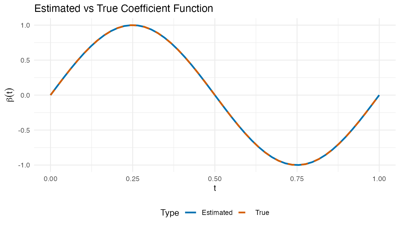

Nonparametric Regression (fregre.np)

Nonparametric functional regression makes no parametric assumptions about the relationship between $X(t)$ and $Y$. Instead, it estimates $\mathbb{E}[Y | X = x]$ directly using local averaging techniques.

The General Framework

Given a new functional observation $X^*$, the predicted response is:

$$\hat{Y}^* = \hat{m}(X^*) = \sum_{i=1}^{n} w_i(X^*) Y_i$$

where $w_i(X^*)$ are weights that depend on the “distance” between $X^*$ and the training curves $X_i$.

Nadaraya-Watson Estimator

The Nadaraya-Watson (kernel regression) estimator uses:

$$\hat{m}(X^*) = \frac{\sum_{i=1}^{n} K\left(\frac{d(X^*, X_i)}{h}\right) Y_i}{\sum_{i=1}^{n} K\left(\frac{d(X^*, X_i)}{h}\right)}$$

where $K(\cdot)$ is a kernel function and $h > 0$ is the bandwidth.

Kernel	Formula $K(u)$
Gaussian	$\frac{1}{\sqrt{2\pi}} e^{-u^2/2}$
Epanechnikov	$\frac{3}{4}(1-u^2) \mathbf{1}_{|u| \leq 1}$
Uniform	$\frac{1}{2} \mathbf{1}_{|u| \leq 1}$

k-Nearest Neighbors

The k-NN estimator averages the responses of the $k$ closest curves:

$$\hat{m}(X^*) = \frac{1}{k} \sum_{i \in \mathcal{N}_k(X^*)} Y_i$$

Two variants are available:

• Global k-NN (kNN.gCV): single $k$ selected by leave-one-out CV
• Local k-NN (kNN.lCV): adaptive $k$ that may vary per prediction point

Nadaraya-Watson Example

# Fit nonparametric regression with Nadaraya-Watson
fit_np <- fregre.np(fd, y, type.S = "S.NW")
print(fit_np)
#> Nonparametric functional regression model
#>   Number of observations: 100 
#>   Smoother type: S.NW 
#>   Bandwidth: 0.3302789 
#>   R-squared: 0.0552

k-Nearest Neighbors

# Global k-NN (single k for all observations)
fit_knn_global <- fregre.np(fd, y, type.S = "kNN.gCV")

# Local k-NN (adaptive k per observation)
fit_knn_local <- fregre.np(fd, y, type.S = "kNN.lCV")

cat("Global k-NN optimal k:", fit_knn_global$knn, "\n")
#> Global k-NN optimal k: 20

Bandwidth Selection

# Cross-validation for bandwidth
cv_np <- fregre.np.cv(fd, y, h.range = seq(0.1, 1, by = 0.1))

cat("Optimal bandwidth:", cv_np$optimal.h, "\n")
#> Optimal bandwidth: 0.2

Different Kernels

# Epanechnikov kernel
fit_epa <- fregre.np(fd, y, Ker = "epa")

# Available kernels: "norm", "epa", "tri", "quar", "cos", "unif"

Different Metrics

# Use L1 metric instead of default L2
fit_np_l1 <- fregre.np(fd, y, metric = metric.lp, p = 1)

# Use semimetric based on PCA
fit_np_pca <- fregre.np(fd, y, metric = semimetric.pca, ncomp = 5)

Multiple Functional Predictors

When the response depends on more than one functional predictor, fregre.np.multi() extends nonparametric regression to handle a list of functional predictors.

# Simulate a second functional predictor
set.seed(123)
X2 <- matrix(0, n, m)
for (i in 1:n) {
  X2[i, ] <- cos(2 * pi * t_grid) * rnorm(1, 0, 0.5) +
    rnorm(m, sd = 0.1)
}
fd2 <- fdata(X2, argvals = t_grid)

# Response depends on both predictors
beta_true2 <- cos(4 * pi * t_grid)
y_multi <- numeric(n)
for (i in 1:n) {
  y_multi[i] <- sum(beta_true * X[i, ]) / m +
    0.5 * sum(beta_true2 * X2[i, ]) / m +
    rnorm(1, sd = 0.3)
}

# Fit with multiple functional predictors
fit_multi <- fregre.np.multi(list(fd, fd2), y_multi)
print(fit_multi)
#> Nonparametric functional regression with multiple predictors
#> =============================================================
#> Number of observations: 100 
#> Number of functional predictors: 2 
#> Smoother type: S.NW 
#> Weights: 0.5, 0.5 
#> Bandwidth: 0.2809 
#> R-squared: 0.0632

Mixed Functional and Scalar Predictors

Real datasets often include both functional and scalar covariates. fregre.np.mixed() handles this by selecting separate bandwidths for the functional and scalar parts.

# Add a scalar covariate
z <- rnorm(n)
y_mixed <- y + 0.8 * z  # scalar effect added

# Fit with functional + scalar predictors
fit_mixed <- fregre.np.mixed(fd, y_mixed, scalar.covariates = z)
print(fit_mixed)
#> Nonparametric functional regression model
#>   Number of observations: 100 
#>   Smoother type: 
#>   R-squared: 0.7061

Testing the Linear Model Assumption

Before choosing between linear and nonparametric methods, flm.test() tests whether the functional linear model is adequate. If the null hypothesis (linear relationship) is not rejected, PC and basis regression are justified; otherwise nonparametric methods may be preferable.

# Test H0: the relationship between X(t) and Y is linear
flm_result <- flm.test(fd_train, y_train, B = 200)
print(flm_result)
#> 
#>  Projected Cramer-von Mises test for FLM
#> 
#> data:  
#> = 2073.2, p-value = 0.13

A large p-value supports the linear model; a small p-value ($< 0.05$) suggests the true relationship is nonlinear and parametric methods may be misspecified.

Comparing Methods

# Fit all methods on training data
fit1 <- fregre.pc(fd_train, y_train, ncomp = 3)
fit2 <- fregre.basis(fd_train, y_train, nbasis = 15)
fit3 <- fregre.np(fd_train, y_train, type.S = "S.NW")
fit4 <- fregre.np(fd_train, y_train, type.S = "kNN.gCV")
fit5 <- fregre.lm(fd_train, y_train, ncomp = 3)

# Predict on test data
pred1 <- predict(fit1, fd_test)
pred2 <- predict(fit2, fd_test)
pred3 <- predict(fit3, fd_test)
pred4 <- predict(fit4, fd_test)
pred5 <- predict(fit5, fd_test)

# Compare performance
results <- data.frame(
  Method = c("fregre.pc", "fregre.basis",
             "Nadaraya-Watson", "k-NN", "fregre.lm (Rust)"),
  RMSE = round(c(pred.RMSE(y_test, pred1),
                  pred.RMSE(y_test, pred2),
                  pred.RMSE(y_test, pred3),
                  pred.RMSE(y_test, pred4),
                  pred.RMSE(y_test, pred5)), 4),
  R2 = round(c(pred.R2(y_test, pred1),
                pred.R2(y_test, pred2),
                pred.R2(y_test, pred3),
                pred.R2(y_test, pred4),
                pred.R2(y_test, pred5)), 4),
  MAE = round(c(pred.MAE(y_test, pred1),
                 pred.MAE(y_test, pred2),
                 pred.MAE(y_test, pred3),
                 pred.MAE(y_test, pred4),
                 pred.MAE(y_test, pred5)), 4)
)
knitr::kable(results, caption = "Hold-out test set performance")

Hold-out test set performance

Method	RMSE	R2	MAE
fregre.pc	0.4570	0.2188	0.3820
fregre.basis	0.8990	-2.0226	0.7162
Nadaraya-Watson	0.5359	-0.0742	0.4453
k-NN	0.4935	0.0891	0.4186
fregre.lm (Rust)	11.9563	-533.6283	9.2836

Visualizing Predictions

df_pred <- data.frame(
  Observed = rep(y_test, 5),
  Predicted = c(pred1, pred2, pred3, pred4, pred5),
  Method = rep(c("fregre.pc", "fregre.basis",
                 "Nadaraya-Watson", "k-NN", "fregre.lm"),
               each = length(y_test))
)

ggplot(df_pred, aes(x = Observed, y = Predicted)) +
  geom_point(alpha = 0.7) +
  geom_abline(intercept = 0, slope = 1, linetype = "dashed", color = "red") +
  facet_wrap(~ Method, nrow = 2) +
  labs(title = "Observed vs Predicted by Method",
       x = "Observed", y = "Predicted")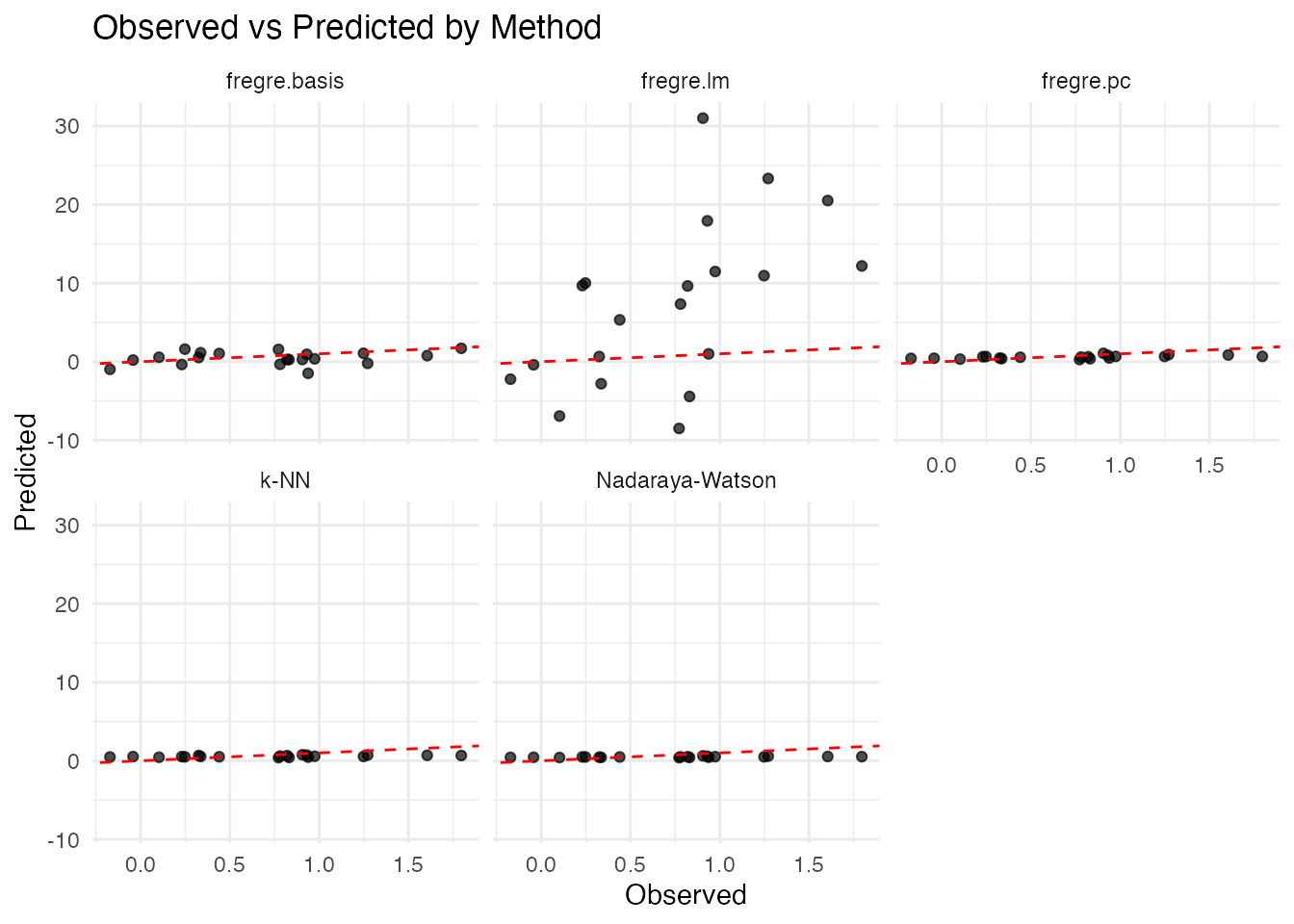

Comparison Table

Method	Model	Key Parameter	Speed	Interpretability
fregre.lm	$Y = \alpha + \sum_k \gamma_k \xi_{ik}$	$K$ (# components)	Fast	High
fregre.pc	$Y = \alpha + \sum_k \gamma_k \xi_{ik}$	$K$ (# components)	Fast	High
fregre.basis	$Y = \alpha + \int \beta(t) X(t) dt$	$\lambda$ (penalty)	Fast	High
fregre.np (NW)	$Y = m(X)$ (nonparametric)	$h$ (bandwidth)	Moderate	Low
fregre.np (kNN)	$Y = \frac{1}{k}\sum_{j \in \mathcal{N}_k} Y_j$	$k$ (neighbors)	Moderate	Low

Model Diagnostics

After fitting a functional linear model, standard regression diagnostics help check whether the model assumptions hold.

Residual Plots

df_diag <- data.frame(
  Fitted = fit_lm$fitted.values,
  Residuals = fit_lm$residuals
)

ggplot(df_diag, aes(x = Fitted, y = Residuals)) +
  geom_point(alpha = 0.6) +
  geom_hline(yintercept = 0, linetype = "dashed", color = "red") +
  labs(title = "Fitted vs Residuals (fregre.lm)",
       x = "Fitted values", y = "Residuals")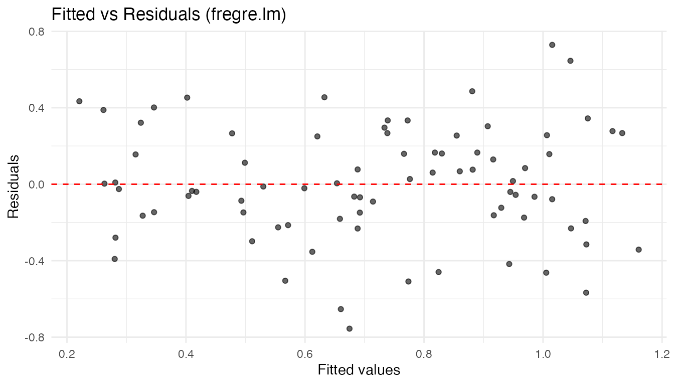

A random scatter around zero supports the linearity and constant-variance assumptions. Fan-shaped or curved patterns suggest heteroscedasticity or nonlinearity.

QQ-Plot of Residuals

ggplot(df_diag, aes(sample = Residuals)) +
  stat_qq(alpha = 0.6) +
  stat_qq_line(color = "red", linetype = "dashed") +
  labs(title = "Normal QQ-Plot of Residuals",
       x = "Theoretical quantiles", y = "Sample quantiles")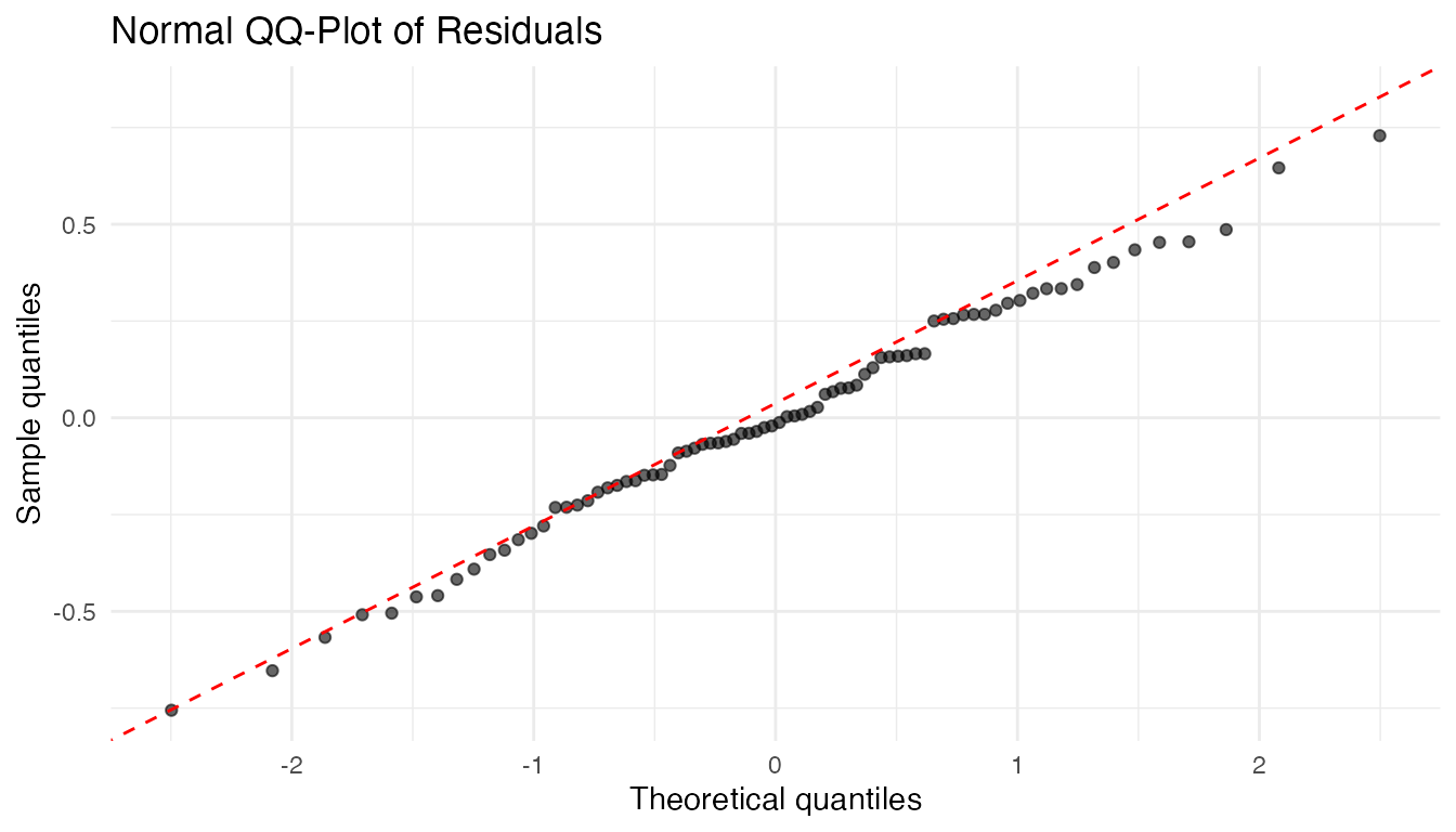

Visualizing Beta(t) with Confidence Bands

# fregre.lm stores beta(t) as an fdata object and SEs from the FPC regression
coefs <- fit_lm$coefficients[-1]  # exclude intercept
loadings <- fit_lm$.fpca_rotation  # m x K matrix of FPC loadings

beta_hat_lm <- as.numeric(loadings %*% coefs)

# Approximate pointwise SE via delta method using FPC score regression SEs
se_coefs <- fit_lm$std.errors[-1]  # exclude intercept SE
beta_se <- sqrt(as.numeric((loadings^2) %*% (se_coefs^2)))

df_beta_ci <- data.frame(
  t = t_lm,
  beta = beta_hat_lm,
  lower = beta_hat_lm - 1.96 * beta_se,
  upper = beta_hat_lm + 1.96 * beta_se,
  true_beta = beta_true_lm
)

ggplot(df_beta_ci, aes(x = t)) +
  geom_ribbon(aes(ymin = lower, ymax = upper), fill = "#0072B2", alpha = 0.2) +
  geom_line(aes(y = beta), color = "#0072B2", linewidth = 1) +
  geom_line(aes(y = true_beta), color = "#D55E00", linetype = "dashed",
            linewidth = 0.8) +
  labs(title = "Estimated Beta(t) with 95% Pointwise Confidence Band",
       x = "t", y = expression(hat(beta)(t))) +
  annotate("text", x = 0.8, y = max(beta_hat_lm) * 0.9,
           label = "True", color = "#D55E00") +
  annotate("text", x = 0.8, y = max(beta_hat_lm) * 0.7,
           label = "Estimated", color = "#0072B2")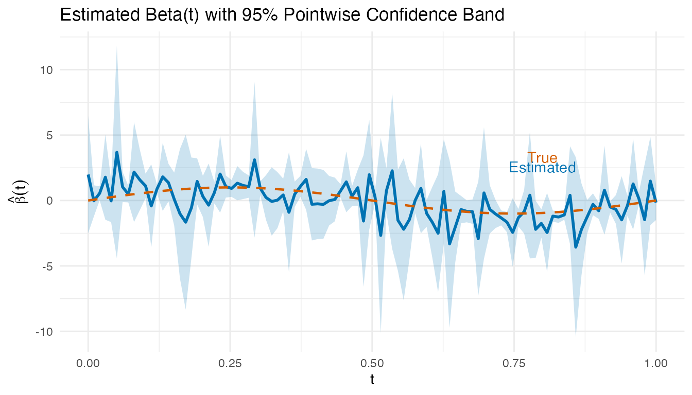

Regions where the confidence band excludes zero indicate time points where the predictor significantly influences the response.

For comprehensive diagnostics (influence, Cook’s distance, DFBETAS, etc.), see vignette("articles/regression-diagnostics").

Prediction Metrics

Model performance is evaluated using standard regression metrics:

Metric	Formula	Interpretation
MAE	$\frac{1}{n}\sum |y_i - \hat{y}_i|$	Average absolute error
MSE	$\frac{1}{n}\sum (y_i - \hat{y}_i)^2$	Average squared error
RMSE	$\sqrt{\text{MSE}}$	Error in original units
$R^2$	$1 - \frac{\sum(y_i - \hat{y}_i)^2}{\sum(y_i - \bar{y})^2}$	Proportion of variance explained

cat("MAE:", pred.MAE(y_test, pred1), "\n")
#> MAE: 0.3819577
cat("MSE:", pred.MSE(y_test, pred1), "\n")
#> MSE: 0.2088714
cat("RMSE:", pred.RMSE(y_test, pred1), "\n")
#> RMSE: 0.4570245
cat("R2:", pred.R2(y_test, pred1), "\n")
#> R2: 0.2188439

All methods support leave-one-out cross-validation (LOOCV) for parameter selection:

$$\text{CV} = \frac{1}{n} \sum_{i=1}^{n} (Y_i - \hat{Y}_{-i})^2$$

This is implemented efficiently using the “hat matrix trick” for linear methods.

Practical Workflow

A recommended workflow for scalar-on-function regression:

1. Start simple: fit fregre.lm.cv() to find the optimal number of FPC components via cross-validation.
2. Check linearity: run flm.test() on the training data. A significant p-value suggests nonlinearity.
3. If linear holds: compare fregre.lm(), fregre.pc(), and fregre.basis() — all estimate the functional linear model with different regularization strategies.
4. If linearity is rejected: try fregre.np() with bandwidth cross-validation (fregre.np.cv()).
5. Evaluate: hold out a test set and compare methods with pred.RMSE(), pred.R2(), and pred.MAE().
6. Diagnose: check residual plots and the estimated $\hat{\beta}(t)$ for interpretability.

set.seed(42)
tr <- sample(n, 70)
te <- setdiff(1:n, tr)

fd_tr <- fd[tr, ]
fd_te <- fd[te, ]
y_tr <- y[tr]
y_te <- y[te]

# Step 1: CV for component selection
cv <- fregre.lm.cv(fd_tr, y_tr, k.range = 1:6, nfold = 5)

# Step 2: Test linearity
linearity <- flm.test(fd_tr, y_tr, B = 200)
cat("FLM test p-value:", linearity$p.value, "\n")
#> FLM test p-value: 0.65

# Step 3-4: Fit best linear and nonparametric
fit_best_lm <- fregre.lm(fd_tr, y_tr, ncomp = cv$optimal.k)
fit_best_np <- fregre.np(fd_tr, y_tr, type.S = "kNN.gCV")

# Step 5: Evaluate
pred_lm_wf <- predict(fit_best_lm, fd_te)
pred_np_wf <- predict(fit_best_np, fd_te)

cat("Linear RMSE:", round(pred.RMSE(y_te, pred_lm_wf), 4),
    "| R2:", round(pred.R2(y_te, pred_lm_wf), 4), "\n")
#> Linear RMSE: 20.2929 | R2: -1967.406
cat("Nonpar RMSE:", round(pred.RMSE(y_te, pred_np_wf), 4),
    "| R2:", round(pred.R2(y_te, pred_np_wf), 4), "\n")
#> Nonpar RMSE: 0.5028 | R2: -0.2086

Method Selection Guide

FPC Regression (fregre.lm / fregre.pc):

• Best when the functional predictor has clear dominant modes of variation
• Computationally efficient for large datasets
• Interpretable: each PC represents a pattern in the data
• fregre.lm() is the only model with full explainability support

Basis Expansion Regression (fregre.basis):

• Best when you believe $\beta(t)$ is smooth
• Use B-splines for local features, Fourier for periodic patterns
• The penalty parameter $\lambda$ provides automatic regularization
• Good when you want to visualize and interpret $\hat{\beta}(t)$

Nonparametric Regression (fregre.np):

• Best when the relationship between $X$ and $Y$ may be nonlinear
• Makes minimal assumptions about the data-generating process
• Computationally more expensive (requires distance calculations)
• May require larger sample sizes for stable estimation

See Also

• vignette("articles/function-on-scalar") — when the response is a curve
• vignette("articles/elastic-regression") — alignment-aware regression
• vignette("articles/functional-classification") — classifying curves (including functional.logistic())
• vignette("articles/explainability") — interpreting fregre.lm() models
• vignette("articles/regression-diagnostics") — influence, Cook’s distance, VIF
• vignette("articles/uncertainty-quantification") — prediction intervals
• vignette("articles/cross-validation") — cross-validation framework
• vignette("fpca", package = "fdars") — functional principal component analysis
• vignette("basis-representation", package = "fdars") — basis function representations

References

Foundational texts:

• Ramsay, J.O. and Silverman, B.W. (2005). Functional Data Analysis, 2nd ed. Springer.
• Ferraty, F. and Vieu, P. (2006). Nonparametric Functional Data Analysis: Theory and Practice. Springer.
• Horváth, L. and Kokoszka, P. (2012). Inference for Functional Data with Applications. Springer.

Key methodological papers:

• Cardot, H., Ferraty, F., and Sarda, P. (1999). Functional Linear Model. Statistics & Probability Letters, 45(1), 11–22.
• Reiss, P.T. and Ogden, R.T. (2007). Functional Principal Component Regression and Functional Partial Least Squares. Journal of the American Statistical Association, 102(479), 984–996.
• Goldsmith, J., Bobb, J., Crainiceanu, C., Caffo, B., and Reich, D. (2011). Penalized Functional Regression. Journal of Computational and Graphical Statistics, 20(4), 830–851.
• Ferraty, F., Laksaci, A., and Vieu, P. (2006). Estimating Some Characteristics of the Conditional Distribution in Nonparametric Functional Models. Statistical Inference for Stochastic Processes, 9, 47–76.