Elastic Regression

Introduction

Functional regression often assumes curves are meaningfully aligned before analysis. However, when functional predictors contain phase variability (differences in timing or alignment), standard regression methods blend amplitude and phase variation, reducing predictive power and interpretability of the coefficient function.

Elastic regression addresses this by jointly estimating the alignment warping functions and regression coefficients, separating phase from amplitude variation.

Elastic Regression: Joint Alignment + Prediction

Mathematical Framework

Standard Functional Linear Model

The scalar-on-function model is

$y_i = \alpha + \int_0^1 X_i(t)\,\beta(t)\,\mathrm{d}t + \varepsilon_i.$

When curves $X_i$ are misaligned, the integral mixes amplitude and phase effects, and the estimated $\hat{\beta}(t)$ becomes blurred and uninterpretable.

Elastic Regression Model

Elastic regression introduces warping functions $\gamma_i \in \Gamma$ :

$y_i = \alpha + \int_0^1 \tilde{X}_i(t)\,\beta(t)\,\mathrm{d}t + \varepsilon_i, \qquad \tilde{X}_i = X_i \circ \gamma_i.$

The algorithm alternates between:

Alignment step: Fix $\beta(t)$ , update warping functions $\gamma_i$ to minimize the residual sum of squares via the Fisher-Rao elastic metric.
Regression step: Fix warping functions, re-estimate $\alpha$ and $\beta(t)$ from the aligned curves.

Convergence is measured by the relative change in SSE. The SRVF representation $q_i = \text{SRVF}(\tilde{X}_i)$ ensures the alignment respects the elastic geometry (Srivastava et al., 2011).

Elastic Logistic Model

For binary classification $y_i \in \{0,1\}$ , the model becomes

$\log\frac{P(y_i = 1)}{P(y_i = 0)} = \alpha + \int_0^1 \tilde{X}_i(t)\,\beta(t)\,\mathrm{d}t,$

with the same alternating alignment-regression optimization.

Elastic PCR

Elastic Principal Component Regression first computes elastic FPCA scores (vertical, horizontal, or joint), then regresses $y$ on the scores:

$y_i = \alpha + \sum_{k=1}^{K} b_k\,\xi_{ik} + \varepsilon_i,$

where $\xi_{ik}$ are scores from the chosen FPCA mode.

Simulated Data: Warped Template with Amplitude Signal

We simulate a scenario that strongly favours elastic regression: all curves share a common shape (template), but each is nonlinearly warped by a random diffeomorphism. The response depends on a subtle amplitude perturbation that is invisible to standard FPCA because the dominant variation is phase:

n <- 60
m <- 80
t <- seq(0, 1, length.out = m)

template <- function(s) sin(2 * pi * s) + 0.3 * sin(6 * pi * s)

X <- matrix(0, n, m)
y <- numeric(n)
for (i in 1:n) {
  # Random nonlinear warp via Beta CDF
  a <- runif(1, 0.5, 2.0)
  b <- runif(1, 0.5, 2.0)
  gamma <- pbeta(t, a, b)

  # Amplitude perturbation (the signal)
  delta <- rnorm(1, 0, 0.4)

  # Warped and scaled template
  X[i, ] <- (1 + 0.2 * delta) *
            approx(t, template(t), xout = gamma, rule = 2)$y +
            rnorm(m, sd = 0.1)

  # Response depends on amplitude perturbation
  y[i] <- 2 * delta + rnorm(1, sd = 0.3)
}
fd <- fdata(X, argvals = t)

plot(fd, main = "Functional Predictors: Nonlinearly Warped Template",
     xlab = "t", ylab = "X(t)")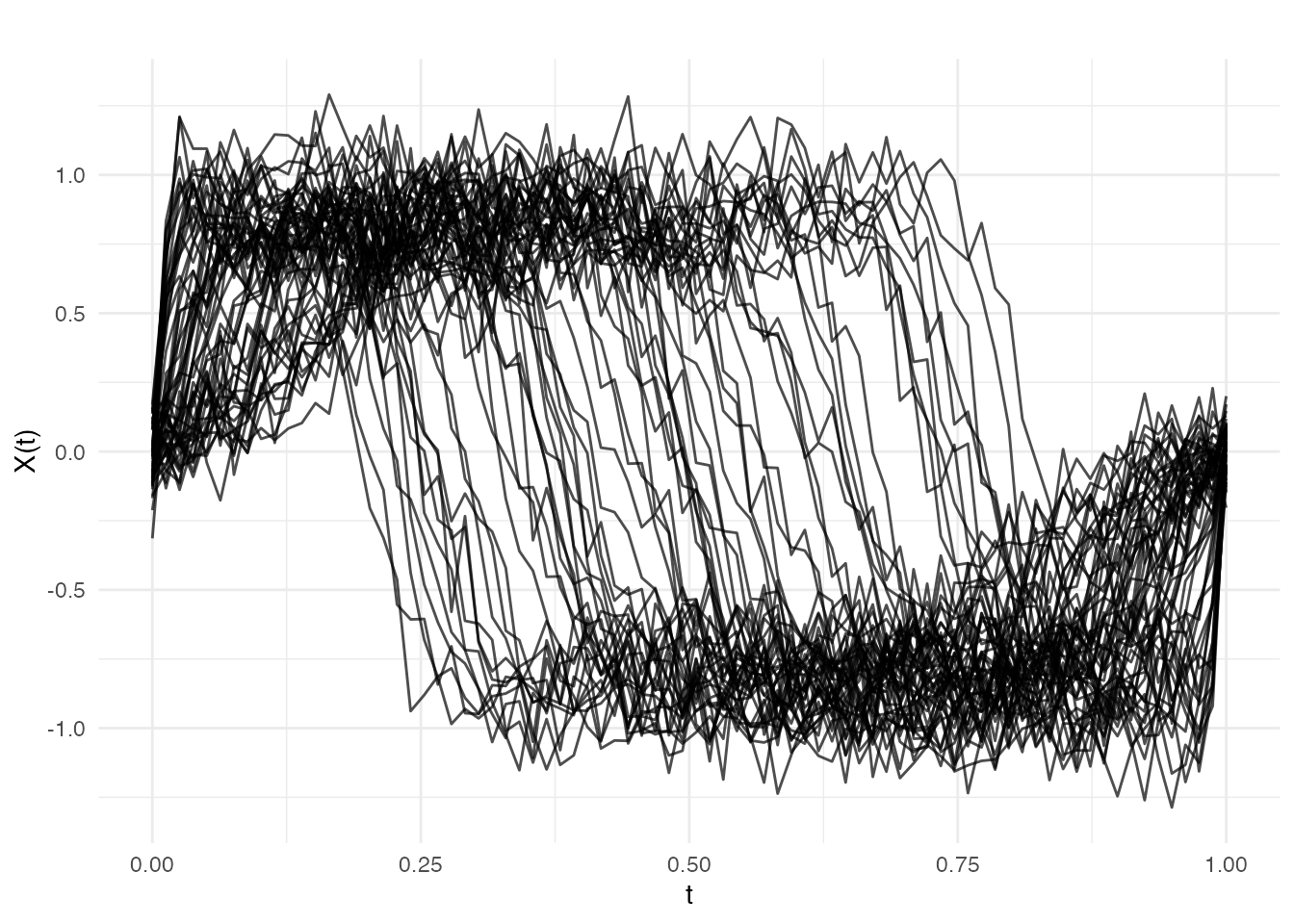

Standard FPCA spends nearly all its components capturing the dominant warp variation, leaving little capacity for the amplitude signal that drives the response.

Standard Regression (Baseline)

fit_std <- fregre.lm(fd, y, ncomp = 5)
cat("Standard fregre.lm R\u00b2:", round(fit_std$r.squared, 4), "\n")
#> Standard fregre.lm R²: 0.1015

df_std <- data.frame(Observed = y, Fitted = fit_std$fitted.values)
ggplot(df_std, aes(x = Observed, y = Fitted)) +
  geom_point(color = "#4A90D9", size = 2.5, alpha = 0.7) +
  geom_abline(slope = 1, intercept = 0, linetype = "dashed", color = "gray50") +
  labs(title = "Standard Regression: Observed vs Fitted",
       subtitle = paste("R\u00b2 =", round(fit_std$r.squared, 3)),
       x = "Observed", y = "Fitted")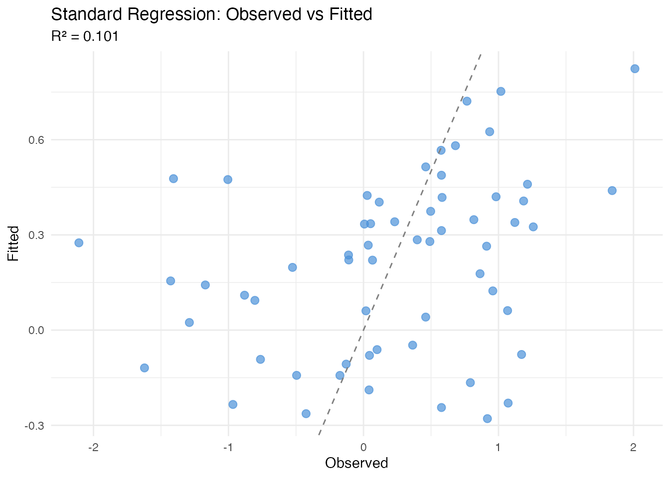

Standard regression fails because the FPCs capture warp variation rather than the amplitude signal the response depends on.

Elastic Scalar-on-Function Regression

elastic.regression() jointly estimates alignment and regression, removing the phase variation before fitting:

fit_elastic <- elastic.regression(fd, y, ncomp.beta = 5, lambda = 0.01,
                                  max.iter = 20, tol = 1e-3)
cat("Elastic regression R\u00b2:", round(fit_elastic$r.squared, 4), "\n")
#> Elastic regression R²: 0.868
cat("Iterations:", fit_elastic$n.iter, "\n")
#> Iterations: 20

plot(fit_elastic, type = "fit")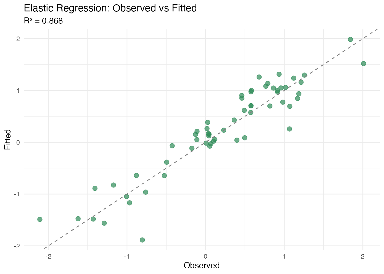

plot(fit_elastic, type = "beta")

plot(fit_elastic, type = "residuals")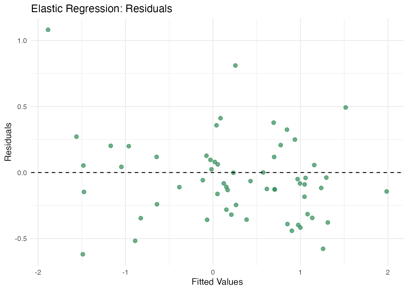

Comparison

comp <- data.frame(
  Method = c("Standard (fregre.lm)", "Elastic Regression"),
  R2 = c(fit_std$r.squared, fit_elastic$r.squared),
  RMSE = c(sqrt(mean(fit_std$residuals^2)),
           sqrt(mean(fit_elastic$residuals^2)))
)
print(comp)
#>                 Method        R2      RMSE
#> 1 Standard (fregre.lm) 0.1014741 0.8171993
#> 2   Elastic Regression 0.8680056 0.3132134

Elastic Logistic Classification

For binary classification:

y_bin <- as.numeric(y > median(y))

fit_logistic <- elastic.logistic(fd, y_bin, ncomp.beta = 5, lambda = 0.01,
                                 max.iter = 15, tol = 1e-3)
cat("Accuracy:", round(fit_logistic$accuracy * 100, 1), "%\n")
#> Accuracy: 98.3 %

plot(fit_logistic, type = "probabilities")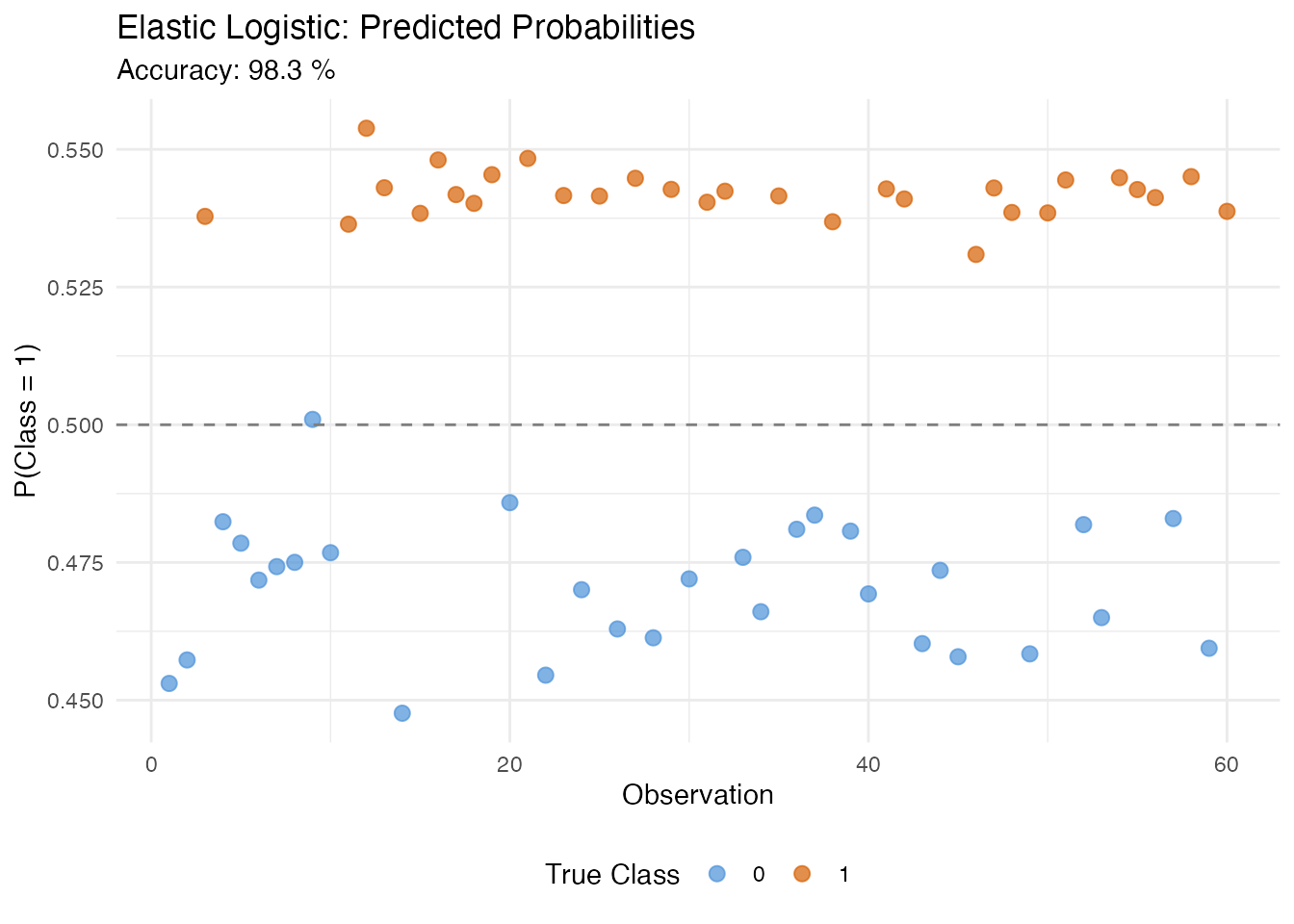

Elastic PCR

Compare vertical, horizontal, and joint PCA methods:

fit_vert <- elastic.pcr(fd, y, ncomp = 3, pca.method = "vertical")
fit_horiz <- elastic.pcr(fd, y, ncomp = 3, pca.method = "horizontal")
fit_joint <- elastic.pcr(fd, y, ncomp = 3, pca.method = "joint")

comp_pcr <- data.frame(
  Method = c("Vertical", "Horizontal", "Joint"),
  R2 = c(fit_vert$r.squared, fit_horiz$r.squared, fit_joint$r.squared)
)
print(comp_pcr)
#>       Method         R2
#> 1   Vertical 0.06631723
#> 2 Horizontal 0.01171428
#> 3      Joint 0.06631723

plot(fit_joint, type = "fit")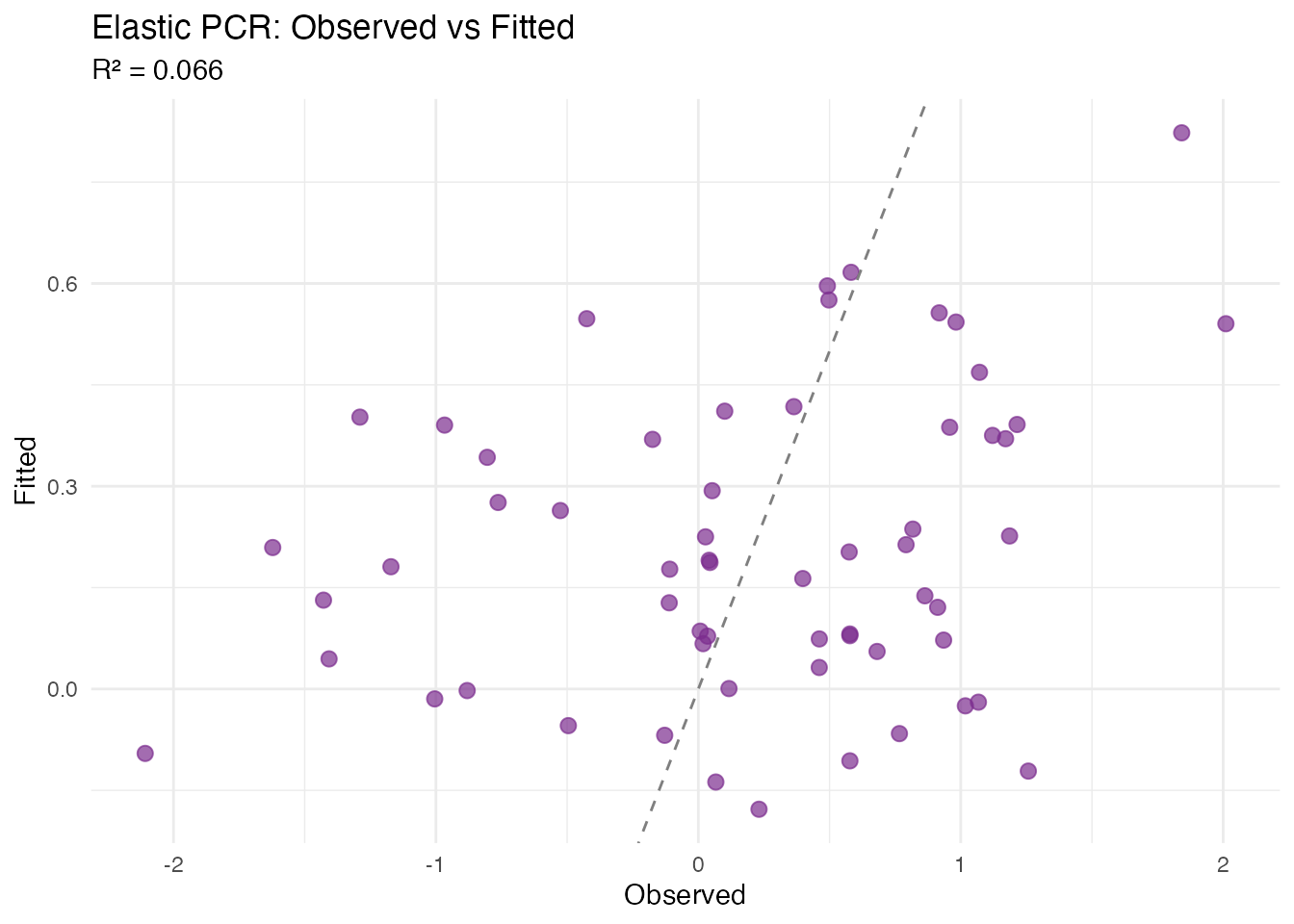

plot(fit_joint, type = "coefficients")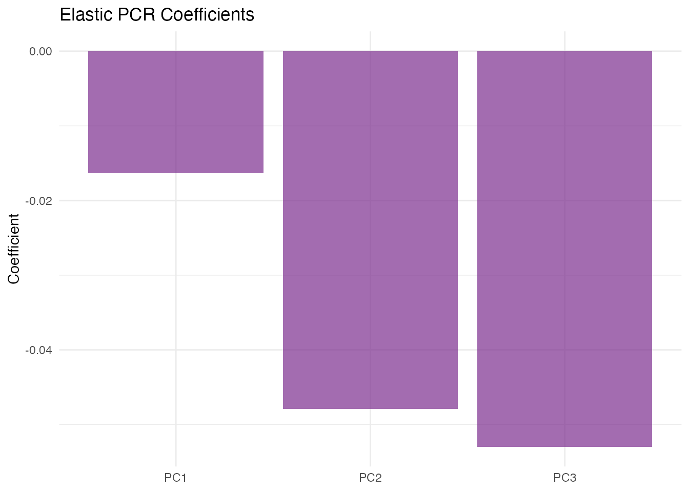

Amplitude vs Phase Attribution

elastic.attribution() quantifies how much of the prediction accuracy is attributable to amplitude variation (shape after alignment) versus phase variation (warping), using elastic PCR scores. This helps decide whether alignment is worthwhile for a given dataset.

attr <- elastic.attribution(fd, y, ncomp = 3, pca.method = "vertical",
                            n.perm = 50, seed = 42)

cat("Amplitude importance:", round(attr$amplitude_importance, 4), "\n")
#> Amplitude importance: 0.1163
cat("Phase importance:", round(attr$phase_importance, 4), "\n")
#> Phase importance: 0

df_attr <- data.frame(
  Source = c("Amplitude", "Phase"),
  Importance = c(attr$amplitude_importance, attr$phase_importance)
)

ggplot(df_attr, aes(x = Source, y = Importance, fill = Source)) +
  geom_col(alpha = 0.7) +
  scale_fill_manual(values = c("Amplitude" = "#4A90D9", "Phase" = "#D55E00")) +
  labs(title = "Amplitude vs Phase Attribution",
       subtitle = "Relative contribution to prediction",
       y = "Importance") +
  theme(legend.position = "none")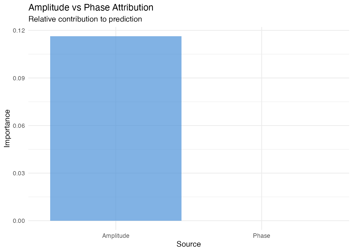

In our simulated data, the response depends on amplitude perturbations, so elastic.attribution() correctly identifies amplitude as the dominant predictive source.

When to Use Elastic Regression

Phase variability dominates: when nonlinear warping is the primary source of variation, standard FPCA wastes components on phase
Interpretability important: want a clear coefficient function after removing phase
Classification with misalignment: use elastic.logistic() for groups with different peak timings
Attribution needed: elastic.attribution() can quantify amplitude vs phase contributions before committing to a full elastic model

Avoid elastic regression if curves are already well-aligned or if the response depends on phase variation itself.

References

Srivastava, A., Wu, W., Kurtek, S., Klassen, E. and Marron, J.S. (2011). Registration of functional data using the Fisher-Rao metric. arXiv preprint arXiv:1103.3817.
Tucker, J.D., Wu, W. and Srivastava, A. (2013). Generative models for functional data using phase and amplitude separation. Computational Statistics & Data Analysis, 61, 50–66.
Ramsay, J.O. and Silverman, B.W. (2005). Functional Data Analysis. 2nd ed. Springer.

Introduction

Mathematical Framework

Standard Functional Linear Model

Elastic Regression Model

Elastic Logistic Model

Elastic PCR

Simulated Data: Warped Template with Amplitude Signal

Standard Regression (Baseline)

Elastic Scalar-on-Function Regression

Comparison

Elastic Logistic Classification

Elastic PCR

Amplitude vs Phase Attribution

When to Use Elastic Regression

References

See Also