Function-on-Scalar Regression

Introduction

Function-on-scalar regression predicts a functional response $Y_i(t)$ from scalar predictors $x_{i1}, \ldots, x_{ip}$. This is the reverse of scalar-on-function regression: the response is a curve, not a number.

Typical questions:

• “How does the treatment shift the entire response curve?”
• “Do group means differ at every time point?”

Mathematical Framework

The function-on-scalar model is:

$$Y_i(t) = \mu(t) + \sum_{j=1}^p x_{ij}\,\beta_j(t) + \varepsilon_i(t)$$

Each coefficient $\beta_j(t)$ is a function describing how predictor $j$ modifies the response curve at each time point $t$. The intercept $\mu(t)$ is the mean response when all predictors are zero.

Penalized Estimation

Direct pointwise OLS at each $t$ would produce coefficient estimates that are noisy and discontinuous. fosr() imposes smoothness via a second-difference roughness penalty:

$$\sum_{i=1}^n \|Y_i - \mu - X_i\beta\|^2 + \lambda \sum_{j=1}^p \int [\beta_j''(t)]^2\,dt$$

where $\lambda > 0$ controls the trade-off between fidelity to the data and smoothness. The solution at each grid point is a ridge-type estimator:

$$\hat\beta(\cdot) = (X^TX + \lambda D^TD)^{-1} X^T Y(\cdot)$$

Pointwise R-squared

The goodness of fit is measured by:

$$R^2(t) = 1 - \frac{\sum_i [Y_i(t) - \hat{Y}_i(t)]^2}{\sum_i [Y_i(t) - \bar{Y}(t)]^2}$$

Values near 1 everywhere indicate the scalar predictors explain the functional response well at all time points; regions with low $R^2(t)$ suggest additional predictors or nonlinear effects may be needed.

Penalized FOSR (fosr)

fosr() estimates the coefficient functions $\beta_j(t)$ with an optional ridge penalty.

set.seed(42)
n <- 60
m <- 80
t_grid <- seq(0, 1, length.out = m)

# Two scalar predictors: treatment and age
treatment <- rep(c(0, 1), each = n/2)
age <- rnorm(n)
predictors <- cbind(treatment, age)

# Functional response depends on predictors
Y <- matrix(0, n, m)
for (i in 1:n) {
  Y[i, ] <- sin(2 * pi * t_grid) +
    treatment[i] * 0.5 * cos(2 * pi * t_grid) +
    age[i] * 0.2 * t_grid +
    rnorm(m, sd = 0.15)
}

fd_y <- fdata(Y, argvals = t_grid)
fosr_fit <- fosr(fd_y, predictors, lambda = 0.1)
print(fosr_fit)
#> Function-on-Scalar Regression
#> =============================
#>   Number of observations: 60 
#>   Number of predictors: 2 
#>   Evaluation points: 80 
#>   R-squared: 0.6412 
#>   Lambda: 0.1

The treatment coefficient $\hat\beta_1(t)$ should recover the simulated $0.5\cos(2\pi t)$ pattern, while the age coefficient $\hat\beta_2(t)$ should approximate the linear $0.2t$ trend.

Visualizing Coefficient Functions

plot(fosr_fit)

Each panel shows one coefficient function $\hat\beta_j(t)$. The shape reveals when during the functional domain each predictor has its strongest effect.

FPC-Based FOSR (fosr.fpc)

fosr.fpc() uses functional principal components instead of penalization:

fosr_fpc_fit <- fosr.fpc(fd_y, predictors, ncomp = 5)
cat("FPC-based R-squared:", round(fosr_fpc_fit$r.squared, 4), "\n")
#> FPC-based R-squared: 0.6421

The FPC-based approach avoids choosing $\lambda$ but requires selecting the number of components. When the response curves have strong low-rank structure (most variance in a few FPCs), this approach is efficient and stable.

Prediction

new_pred <- matrix(c(1, 0.5,   # treated, average age
                     0, -1.0), # control, young
                   nrow = 2, byrow = TRUE)
pred <- predict(fosr_fit, new_pred)

Functional ANOVA (fanova)

Functional ANOVA tests whether the mean functions of $G$ groups are equal:

$$H_0: \mu_1(t) = \mu_2(t) = \cdots = \mu_G(t) \quad \text{for all } t$$

Pointwise F-Statistic

At each grid point $t$:

$$F(t) = \frac{\sum_{g=1}^G n_g [\bar{Y}_g(t) - \bar{Y}(t)]^2 / (G - 1)}{\sum_{g=1}^G \sum_{i \in g} [Y_i(t) - \bar{Y}_g(t)]^2 / (N - G)}$$

These are summarized into a global test statistic by integration:

$$F_{\text{global}} = \int F(t)\,dt$$

Permutation Testing

Because the null distribution of $F_{\text{global}}$ is intractable, fanova() uses a permutation approach:

1. Compute the observed $F_{\text{obs}}$ from the original data.
2. For $b = 1, \ldots, B$: randomly permute group labels and compute $F_b^*$.
3. The p-value is:

$$p = \frac{1 + \#\{F_b^* \geq F_{\text{obs}}\}}{B + 1}$$

This makes the test exact (valid at any sample size) and assumption-free regarding the distribution of $\varepsilon_i(t)$.

Example

set.seed(42)
n_per_group <- 25
m_a <- 80
t_a <- seq(0, 1, length.out = m_a)

# Three treatment groups with different mean functions
Y_anova <- matrix(0, 3 * n_per_group, m_a)
for (i in 1:n_per_group) {
  Y_anova[i, ] <- sin(2 * pi * t_a) + rnorm(m_a, sd = 0.15)
  Y_anova[n_per_group + i, ] <- sin(2 * pi * t_a) +
    0.5 * cos(2 * pi * t_a) + rnorm(m_a, sd = 0.15)
  Y_anova[2 * n_per_group + i, ] <- 2 * t_a - 1 + rnorm(m_a, sd = 0.15)
}
groups <- rep(1:3, each = n_per_group)

fd_anova <- fdata(Y_anova, argvals = t_a)
anova_result <- fanova(fd_anova, groups, n.perm = 500)
print(anova_result)
#> Functional ANOVA
#> ================
#>   Number of groups: 3 
#>   Number of observations: 75 
#>   Global F-statistic: 577.3765 
#>   P-value: 0.001996 
#>   Permutations: 500

A small p-value rejects the null hypothesis that all groups share the same mean function. In this simulation, the three groups have clearly different shapes (sine, sine + cosine, linear), so we expect strong rejection.

Visualizing Group Means

plot(anova_result)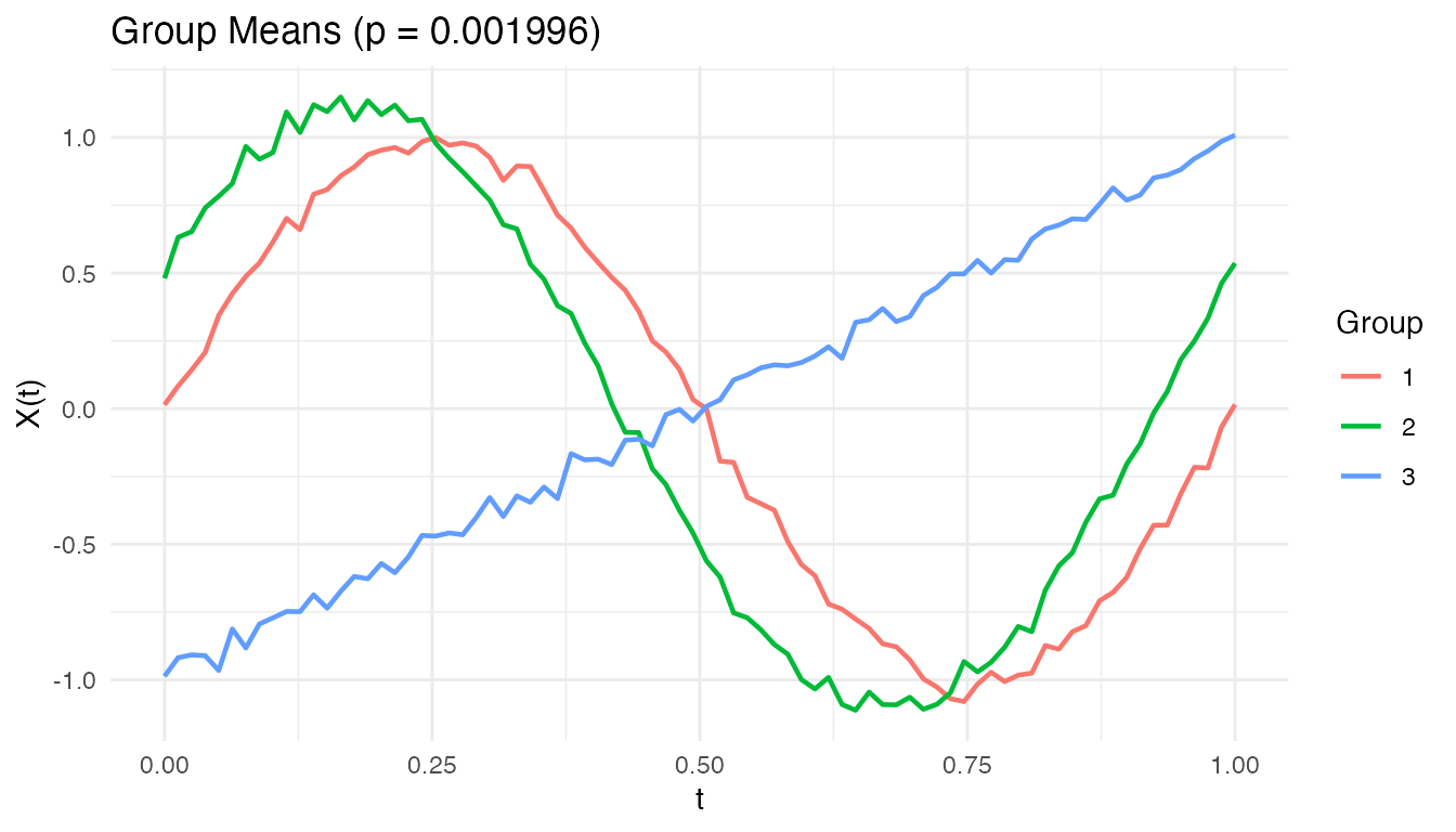

The group mean curves show the estimated $\hat\mu_g(t)$ for each group. Where the curves separate most, the pointwise F-statistic is largest.

Model Diagnostics

After fitting a FOSR model, examine the residuals to check for misspecification. Large residuals concentrated at certain time points suggest the model misses structure there.

# Pointwise residual variance
resid_mat <- fosr_fit$residuals$data
resid_var <- apply(resid_mat, 2, var)

df_resid <- data.frame(t = t_grid, variance = resid_var)
ggplot(df_resid, aes(x = t, y = variance)) +
  geom_line(color = "#0072B2", linewidth = 1) +
  labs(title = "Pointwise Residual Variance",
       x = "t", y = "Var(residual)")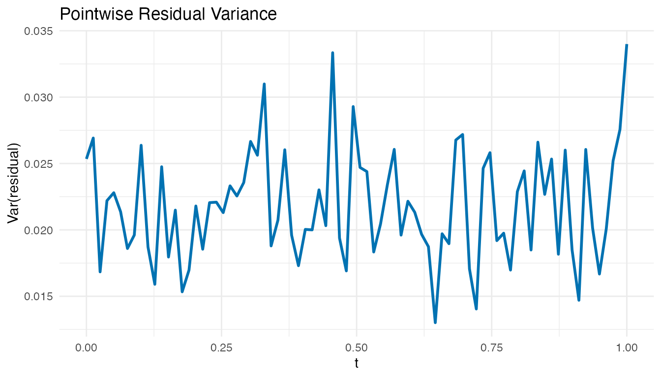

Roughly constant residual variance across $t$ supports the model. Peaks indicate time points where the scalar predictors fail to capture the response variation, suggesting additional predictors or a more flexible model.

2D Function-on-Scalar Regression (fosr.2d)

When the functional response is a 2D surface $Y_i(s, t)$ rather than a curve $Y_i(t)$, standard FOSR does not apply directly. Examples include:

• Spatial-temporal fields — temperature or precipitation measured on a spatial grid over time.
• Brain imaging — cortical activation surfaces from fMRI or EEG.
• Environmental monitoring — pollutant concentrations over a geographic region.

fosr.2d() extends the penalized FOSR framework to surface-valued responses.

Mathematical Model

The 2D function-on-scalar model is:

$$Y_i(s, t) = \mu(s, t) + \sum_{j=1}^p x_{ij}\,\beta_j(s, t) + \varepsilon_i(s, t)$$

Each coefficient $\beta_j(s, t)$ is now a coefficient surface describing how predictor $j$ modifies the response across the entire 2D domain. The intercept $\mu(s, t)$ is the mean surface when all predictors are zero.

Anisotropic Penalization

The two grid directions may require different amounts of smoothing. fosr.2d() supports separate penalties $\lambda_s$ and $\lambda_t$ for the $s$ and $t$ dimensions respectively. This anisotropic penalization is important when the response varies more rapidly in one direction than the other — for example, spatial fields that are smooth geographically but fluctuate quickly over time.

Worked Example

We simulate $n = 40$ observations of a surface response on a $15 \times 15$ grid with two scalar predictors: a continuous predictor x1 and a binary predictor x2.

set.seed(42)
n_2d <- 40
m1 <- 15; m2 <- 15
s_grid <- seq(0, 1, length.out = m1)
t_2d_grid <- seq(0, 1, length.out = m2)

# Two scalar predictors
x1 <- rnorm(n_2d)
x2 <- rbinom(n_2d, 1, 0.5)
pred_2d <- cbind(x1, x2)

# True coefficient surfaces
beta1_true <- outer(s_grid, t_2d_grid, function(s, t)
  0.5 * sin(2 * pi * s) * cos(2 * pi * t))
beta2_true <- outer(s_grid, t_2d_grid, function(s, t)
  exp(-((s - 0.5)^2 + (t - 0.5)^2) / 0.1))

# Generate surface responses (each row is a flattened m1*m2 surface)
Y_2d <- matrix(0, n_2d, m1 * m2)
for (i in 1:n_2d) {
  surface <- sin(pi * outer(s_grid, t_2d_grid, "+")) +
    x1[i] * beta1_true + x2[i] * beta2_true
  Y_2d[i, ] <- as.vector(surface) + rnorm(m1 * m2, sd = 0.1)
}

fd_2d <- fdata(Y_2d)
fit_2d <- fosr.2d(fd_2d, pred_2d, s_grid, t_2d_grid,
                  lambda.s = 0.01, lambda.t = 0.01)
print(fit_2d)
#> 2D Function-on-Scalar Regression
#>   Grid: 15 x 15 
#>   Predictors: 2 
#>   R-squared: 0.7596 
#>   Lambda (s, t): 0.01 , 0.01

Prediction on New Data

Use predict() to obtain fitted surfaces for new observations:

new_pred_2d <- matrix(c(1.0, 1,    # x1 = 1.0, x2 = 1
                         -0.5, 0),  # x1 = -0.5, x2 = 0
                       nrow = 2, byrow = TRUE)
pred_2d_out <- predict(fit_2d, new_pred_2d)

Visualizing Coefficient Surfaces

Each estimated coefficient $\hat\beta_j(s, t)$ is stored as a flattened row in fit_2d$beta$data. To visualize, reshape to the original $m_1 \times m_2$ grid and plot as a heatmap.

# Extract and reshape coefficient surfaces for visualization
coef_list <- list(
  data.frame(
    s = rep(s_grid, m2), t = rep(t_2d_grid, each = m1),
    value = as.vector(matrix(fit_2d$intercept$data[1, ], m1, m2)),
    coefficient = "Intercept"
  ),
  data.frame(
    s = rep(s_grid, m2), t = rep(t_2d_grid, each = m1),
    value = as.vector(matrix(fit_2d$beta$data[1, ], m1, m2)),
    coefficient = "x1"
  ),
  data.frame(
    s = rep(s_grid, m2), t = rep(t_2d_grid, each = m1),
    value = as.vector(matrix(fit_2d$beta$data[2, ], m1, m2)),
    coefficient = "x2"
  )
)
df_coef <- do.call(rbind, coef_list)

ggplot(df_coef, aes(x = .data$s, y = .data$t, fill = .data$value)) +
  geom_tile() +
  facet_wrap(~ .data$coefficient, scales = "free") +
  scale_fill_viridis_c() +
  labs(title = "Estimated Coefficient Surfaces",
       x = "s", y = "t", fill = "Value")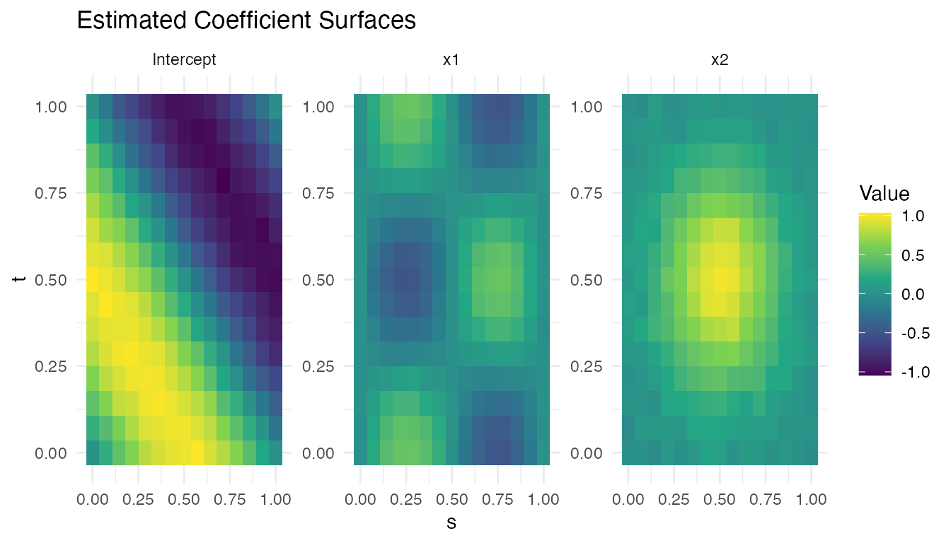

The x1 surface should recover the sinusoidal pattern $0.5\sin(2\pi s)\cos(2\pi t)$, while the x2 surface should approximate the Gaussian bump centred at $(0.5, 0.5)$.

GCV for Tuning

The returned object includes a generalized cross-validation criterion (fit_2d$gcv) that can guide the choice of $\lambda_s$ and $\lambda_t$. Lower GCV values indicate a better bias–variance trade-off. In practice, you can search over a grid of penalty pairs and select the combination that minimizes GCV.

When to Use Each Method

Method	Function	Tuning	Best when
Penalized FOSR	fosr()	$\lambda$	Smooth coefficient functions, large $m$
FPC-Based FOSR	fosr.fpc()	$K$ (# components)	Low-rank response structure
Functional ANOVA	fanova()	$B$ (# permutations)	Testing group differences
2D Penalized FOSR	fosr.2d()	$\lambda_s, \lambda_t$	Surface responses on 2D grids

See Also

• vignette("articles/scalar-on-function") — when the response is a scalar
• vignette("articles/functional-mixed-models") — repeated measures with fmm()
• vignette("articles/example-canadian-weather") — real-data FANOVA + FOSR: regional climate patterns

References

• Ramsay, J.O. and Silverman, B.W. (2005). Functional Data Analysis, 2nd ed. Springer.
• Reiss, P.T. and Ogden, R.T. (2007). Functional Principal Component Regression and Functional Partial Least Squares. Journal of the American Statistical Association, 102(479), 984–996.
• Cuevas, A., Febrero, M., and Fraiman, R. (2004). An anova test for functional data. Computational Statistics & Data Analysis, 47(1), 111–122.