
Methods: Diagnostics & Robustness
Source:vignettes/articles/methods-diagnostics.Rmd
methods-diagnostics.Rmd1. Title & Abstract
This article covers the diagnostics and robustness
tools that validate an event study’s inferential assumptions: residual
normality (Shapiro-Wilk), autocorrelation (Durbin-Watson and Ljung-Box),
pre-event trends, wild-bootstrap inference, and Monte-Carlo power
analysis. After reading, you will know how to check whether the
parametric t-tests are trustworthy for
your data and how to fall back on bootstrap inference when they are not.
All examples run live and offline on earnings_surprises and
simulated data.
2. When to Use This Method
Run diagnostics before trusting any test statistic. Normality and autocorrelation checks tell you whether the parametric CAR t-test’s distributional assumptions hold; a pre-trend test guards against a contaminated estimation window. When assumptions fail, the wild bootstrap provides distribution-free p-values, and a power simulation tells you whether your design could have detected the effect you care about.
3. Intuition
The abnormal-return machinery assumes clean, roughly-normal, serially uncorrelated residuals. Diagnostics interrogate each of those assumptions. If they hold, the closed-form t-tests are fine. If they don’t, resample: the wild bootstrap perturbs the observed abnormal returns with random \pm 1 weights to build an empirical null, sidestepping the normality assumption entirely.
4. Model & Null Hypothesis
Ljung-Box tests residual autocorrelation up to lag h:
Q = n(n+2) \sum_{k=1}^{h} \frac{\hat{\rho}_k^2}{n-k}.
Durbin-Watson targets first-order serial correlation of the residuals e_t (the package computes the approximate statistic directly):
d = \frac{\sum_{t=2}^{n} (e_t - e_{t-1})^2}{\sum_{t=1}^{n} e_t^2}.
The wild bootstrap resamples abnormal returns with Rademacher weights w_b \in \{-1, +1\}:
AR^{*}_{b} = w_b\, \hat{AR}, \qquad w_b \sim \text{Rademacher}.
Power is the Monte-Carlo rejection rate under a specified true effect:
\text{power} = \frac{1}{S}\sum_{s=1}^{S} \mathbf{1}\{\text{reject } H_0 \text{ in sim } s\}.
The null hypotheses are: H_0: \hat{\rho}_k = 0 (no autocorrelation, Ljung-Box / DW d \approx 2) and H_0: \mathbb{E}[AR] = 0 (no abnormal return, bootstrap and power) (Box and Ljung 1978; Durbin and Watson 1950).
5. Assumptions
- Diagnostics are per-event: normality and autocorrelation are checked on each event’s estimation-window residuals.
- DW \approx 2 indicates no first-order autocorrelation; values far from 2 flag it.
- Wild bootstrap relaxes normality but still assumes the abnormal returns are the correct point estimates to resample.
- Power simulation is only as informative as its assumed effect size and noise structure.
6. Worked Example
Diagnostics run live on earnings_surprises; bootstrap
and power run with an explicit seed = 42 for
byte-stability.
library(EventStudy)
data("earnings_surprises")
task   <- EventStudyTask$new(
  earnings_surprises$firm, earnings_surprises$index, earnings_surprises$request
)
params <- ParameterSet$new()
task   <- prepare_event_study(task, params)
task   <- fit_model(task, params)
task   <- calculate_statistics(task, params)
diag <- model_diagnostics(task)   # Shapiro-Wilk, Durbin-Watson, Ljung-Box per event
pt   <- pretrend_test(task)       # pre-event trend test
# Power on a simulated design (zero-network, seed-stable):
sim  <- simulate_event_study(n_events = 20, abnormal_return = 0.02,
                             n_simulations = 200, seed = 42)

# Wild bootstrap inference on the observed task:
boot <- bootstrap_test(task, n_boot = 199, seed = 42)
#> Adding missing grouping variables: `group`
#> Adding missing grouping variables: `group`
7. Rendered Table
es_tt(
  diag,
  caption = "Per-event diagnostics: Shapiro-Wilk (shapiro_p), Durbin-Watson (dw_stat), Ljung-Box (ljung_box_p)."
)| event_id | firm_symbol | is_fitted | shapiro_p | dw_stat | ljung_box_p | acf1 | sigma | r2 |
|---|---|---|---|---|---|---|---|---|
| 1 | AAPL | TRUE | 0.000028141128 | 1.766 | 0.8511 | 0.109 | 0.01065 | 0.7165 |
| 2 | MSFT | TRUE | 0.000000000352 | 1.843 | 0.6812 | 0.07807 | 0.01173 | 0.6901 |
| 3 | GOOGL | TRUE | 0.000000378554 | 1.792 | 0.7391 | 0.09284 | 0.01559 | 0.5945 |
8. Rendered Plot
plot(sim$rejection_by_day$relative_index,
     sim$rejection_by_day$rejection_rate,
     type = "b", pch = 19,
     xlab = "Relative day", ylab = "Rejection rate",
     main = "Simulated power by event-window day")
abline(h = 0.05, lty = 2, col = "grey60")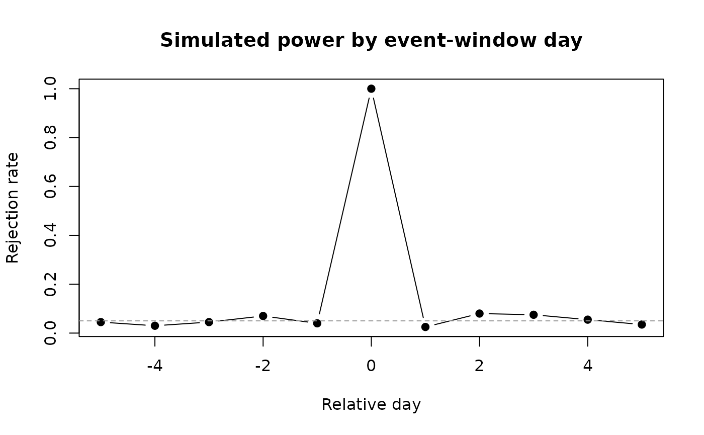
Monte-Carlo rejection rate (power) by event-window day.
9. Interpretation
Read §7 row by row: a small shapiro_p rejects residual
normality (prefer the bootstrap or a nonparametric test); a
dw_stat far from 2 or a small ljung_box_p
flags autocorrelation (inference standard errors are then understated).
The power curve in §8 shows how the design’s detection rate rises around
the event day for the assumed effect — a curve that never lifts much
above the dashed 0.05 line means the study is underpowered for that
effect size. When the diagnostics fail, the wild-bootstrap p-values in boot
(boot_p_aar, boot_p_caar) are the
assumption-light fallback for reporting significance.