Methods: Test Statistics • EventStudy

1. Title & Abstract

This article covers the test statistics EventStudy uses to decide whether average abnormal returns are significantly different from zero. It spans the parametric cross-sectional t-test, the standardized-residual tests of Patell and Boehmer-Musumeci-Poulsen (BMP), the nonparametric sign and rank tests, and the Kolari-Pynnönen (KP) correction for cross-sectional correlation. After reading, you will know which test defends against which failure of the naive t-test, and you will see all five estimated live on the bundled earnings_surprises multi-event panel.

2. When to Use This Method

Cross-sectional t-test (CSectT) — default; assumes independent, homoskedastic abnormal returns across firms.
Patell Z — standardizes each abnormal return by its own forecast-error-corrected estimation-window standard deviation, so noisy firms do not dominate.
BMP t — like Patell but robust to event-induced variance (volatility that rises because of the event).
Sign / rank tests — nonparametric; robust to non-normal, fat-tailed abnormal returns.
Kolari-Pynnönen — corrects BMP for cross-sectional correlation of abnormal returns (e.g. same-industry, same-day events).

3. Intuition

Averaging abnormal returns across firms cancels idiosyncratic noise, leaving the event effect. The tests differ in how they weight and standardize that average: equally (CSectT), by each firm’s own precision (Patell/BMP), by rank or sign (nonparametric), or after netting out the correlation that inflates the naive standard error (KP).

4. Model & Null Hypothesis

The cross-sectional t on the average abnormal return \overline{AR} over N firms:

t = \sqrt{N}\,\frac{\overline{AR}}{s_{AR}}.

Patell Z standardizes each abnormal return by its forecast-error-corrected sigma into a standardized abnormal return SAR_i, then aggregates:

Z = \frac{\sum_i SAR_i}{\sqrt{\sum_i Q_i}}, \qquad Q_i = \frac{m_i - k}{m_i - k - 2},

with m_i estimation-window length and k parameters. BMP replaces the denominator with the cross-sectional standard deviation of the SAR_i, absorbing event-induced variance:

t_{BMP} = \sqrt{N}\,\frac{\overline{SAR}}{s_{SAR}}.

The KP adjustment scales t_{BMP} by the average off-diagonal SAR correlation \bar r:

t_{KP} = t_{BMP}\,\sqrt{\frac{1 - \bar r}{1 + (N-1)\,\bar r}}.

The sign test counts positive abnormal returns w against the null of a fair coin: z = (w - 0.5N)/(0.5\sqrt{N}) (Corrado 1989).

The null hypothesis throughout is H_0: \mathbb{E}[\overline{AR}] = 0 — no average abnormal performance.

5. Assumptions

CSectT: cross-sectionally independent, homoskedastic abnormal returns.
Patell: correct estimation-window sigma; independence across firms.
BMP: relaxes homoskedasticity (handles event-induced variance).
KP: relaxes cross-sectional independence via the correlation correction.
Sign/rank: exchangeability under H_0; no normality required.

6. Worked Example

earnings_surprises is a 3-firm multi-event panel (AAPL / MSFT / GOOGL), which yields average abnormal returns (AAR) and their cumulative counterpart (CAAR). Test statistics are composed as R6 objects and passed into MultiEventStatisticsSet$new().

library(EventStudy)
data("earnings_surprises")

task <- EventStudyTask$new(
  firm_stock_data_tbl = earnings_surprises$firm,
  reference_tbl       = earnings_surprises$index,
  request_tbl         = earnings_surprises$request
)

multi <- MultiEventStatisticsSet$new(tests = list(
  CSectTTest$new(), PatellZTest$new(), BMPTest$new(),
  SignTest$new(), KolariPynnonenTest$new()
))
params <- ParameterSet$new(multi_event_statistics = multi)

task <- prepare_event_study(task, params)
task <- fit_model(task, params)
task <- calculate_statistics(task, params)

Single-event AR/CAR t-tests are available from the default SingleEventStatisticsSet$new() (ARTTest, CARTTest). The family also includes GeneralizedSignTest, the Corrado RankTest, and the CalendarTimePortfolioTest for long-horizon calendar-time inference.

7. Rendered Table

knitr::kable(
  tidy.EventStudyTask(task, type = "aar"),
  caption = "AAR / CAAR with cross-sectional t, plus companion Patell/BMP/Sign/KP statistics."
)

AAR / CAAR with cross-sectional t, plus companion Patell/BMP/Sign/KP statistics.
group	term	estimate	std.error	statistic	p.value	caar	caar_statistic	caar_p.value
Earnings Beat	-5	-0.0048	0.0051	-0.9518	0.4416	-0.0048	-0.9518	0.4416
Earnings Beat	-4	-0.0018	0.0011	-1.6375	0.2432	-0.0066	-1.3184	0.3181
Earnings Beat	-3	0.0064	0.0068	0.9463	0.4439	-0.0003	-0.1398	0.9016
Earnings Beat	-2	0.0021	0.0033	0.6547	0.5799	0.0019	0.5058	0.6633
Earnings Beat	-1	-0.0027	0.0063	-0.4380	0.7041	-0.0009	-0.0886	0.9375
Earnings Beat	0	0.0003	0.0016	0.1690	0.8813	-0.0006	-0.0560	0.9604
Earnings Beat	1	0.0350	0.0218	1.6018	0.2504	0.0344	3.0528	0.0926
Earnings Beat	2	0.0048	0.0033	1.4529	0.2834	0.0392	3.5533	0.0709
Earnings Beat	3	-0.0070	0.0033	-2.1545	0.1640	0.0322	2.4026	0.1382
Earnings Beat	4	-0.0003	0.0027	-0.1177	0.9171	0.0319	2.7628	0.1098
Earnings Beat	5	0.0058	0.0046	1.2728	0.3310	0.0377	2.3509	0.1431

8. Rendered Plot

plot_event_study(task, type = "caar")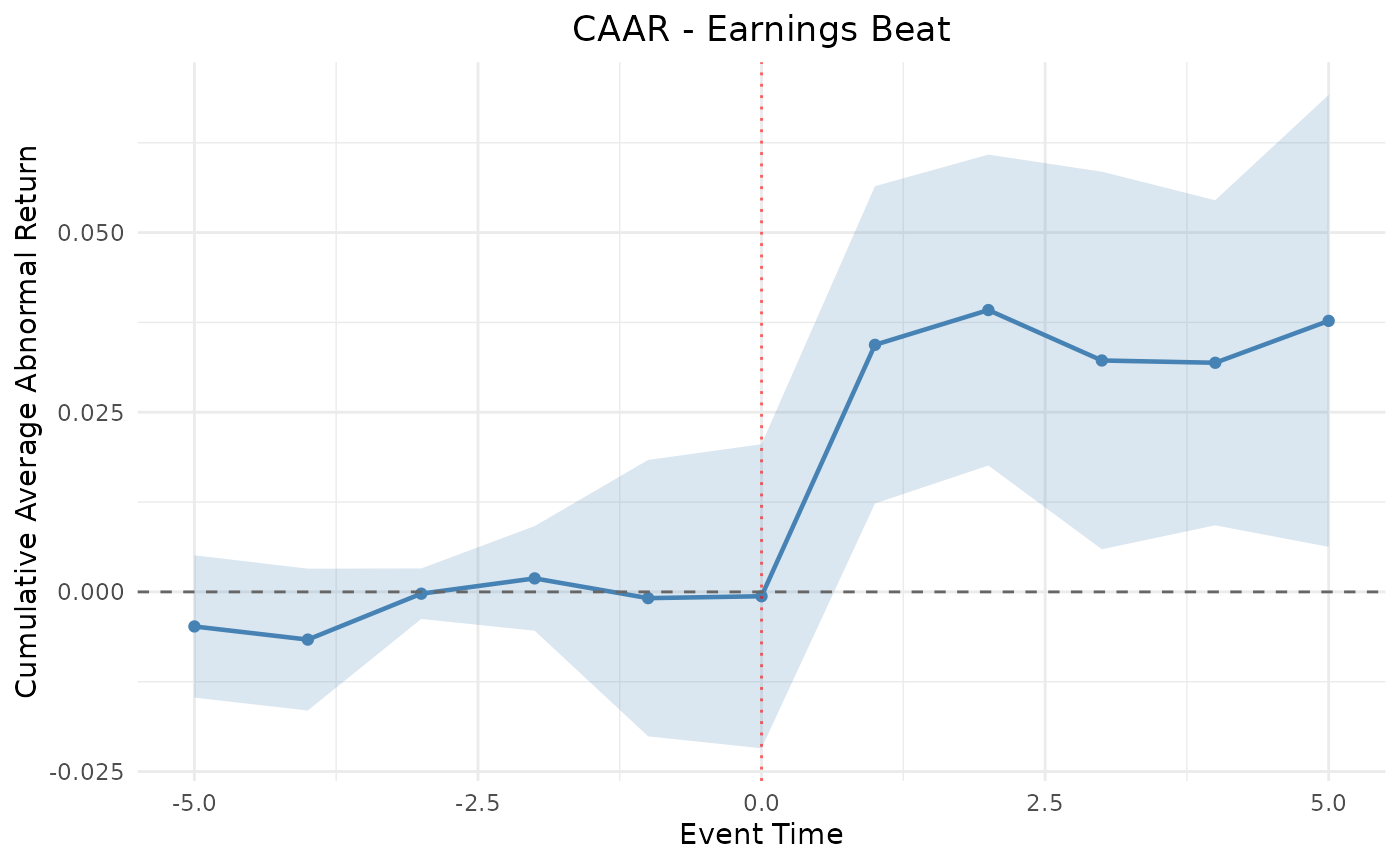

Cumulative average abnormal return (CAAR) across the event window.

9. Interpretation

Each row of §7 reports the AAR at an event-time offset with its cross-sectional t; the CAAR column accumulates them. When the standardized tests (Patell, BMP, KP) diverge from the plain CSectT, that divergence is diagnostic: a large gap between BMP and CSectT points to event-induced variance, while a large KP-vs-BMP gap points to cross-sectional correlation. A significant CAAR that survives KP is the most defensible evidence of an event effect. The plot in §8 shows the CAAR path — a persistent post-event drift is the visual counterpart of a significant cumulative statistic.

References

Corrado, Charles J. 1989. “A Nonparametric Test for Abnormal Security-Price Performance in Event Studies.” Journal of Financial Economics 23 (2): 385–95.