Conformal Prediction for Classification

Introduction

Conformal prediction for classification produces prediction sets — sets of plausible labels with a coverage guarantee — instead of point predictions. For a new observation $x_{\text{new}}$ , the conformal prediction set $C_\alpha(x_{\text{new}})$ satisfies:

$P(y_{\text{new}} \in C_\alpha) \geq 1 - \alpha$

for any distribution, with no assumptions on the data-generating process.

Unlike regression conformal (which produces intervals), classification conformal answers: “which classes are plausible for this observation?” A set of size 1 means high confidence; larger sets indicate ambiguity.

Conformal classification: prediction sets, three methods, and scoring rules

Simulated Data

We simulate a three-class functional classification problem where each class has a distinct mean curve:

n_per_class <- 30
n <- 3 * n_per_class
m <- 50
t_grid <- seq(0, 1, length.out = m)

X <- matrix(0, n, m)
for (i in 1:n_per_class) {
  X[i, ] <- sin(2 * pi * t_grid) + rnorm(m, sd = 0.2)
  X[n_per_class + i, ] <- cos(2 * pi * t_grid) + rnorm(m, sd = 0.2)
  X[2 * n_per_class + i, ] <- 0.5 * t_grid + rnorm(m, sd = 0.2)
}
labels <- rep(1:3, each = n_per_class)

# Train/test split
train_idx <- c(1:25, 31:55, 61:85)
test_idx <- setdiff(1:n, train_idx)

fd_train <- fdata(X[train_idx, ], argvals = t_grid)
fd_test <- fdata(X[test_idx, ], argvals = t_grid)
y_train <- labels[train_idx]
y_test <- labels[test_idx]

df_curves <- data.frame(
  t = rep(t_grid, n),
  value = as.vector(t(X)),
  curve = rep(1:n, each = m),
  class = factor(rep(labels, each = m))
)

ggplot(df_curves, aes(x = .data$t, y = .data$value,
                      group = .data$curve, color = .data$class)) +
  geom_line(alpha = 0.3) +
  labs(title = "Three-Class Functional Data",
       x = "t", y = "X(t)", color = "Class")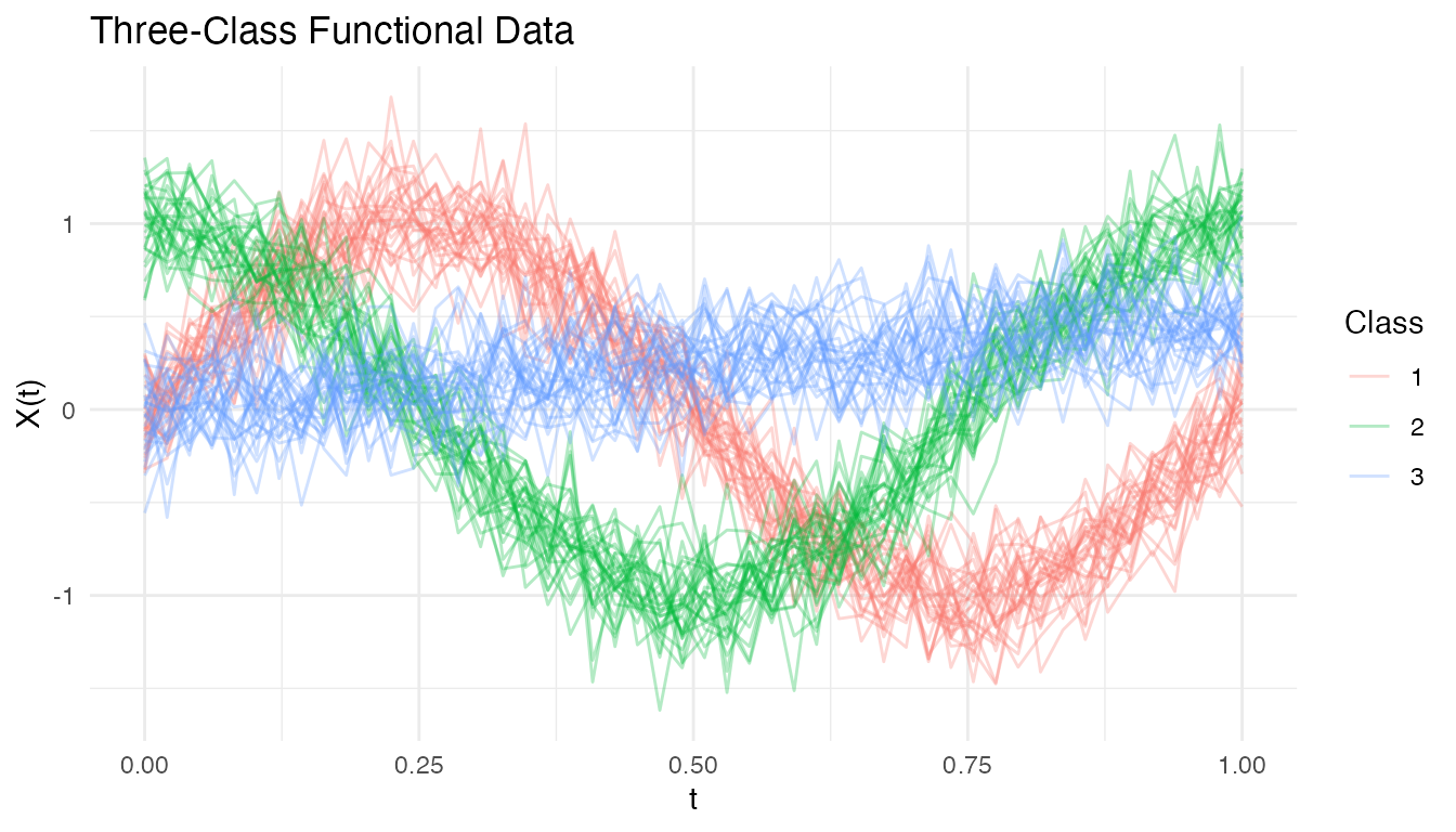

Scoring Rules

Conformal classification uses a nonconformity score to measure how surprising a label is for a given observation. fdars supports two scoring rules:

Score	Name	Description	Set size
LAC	Least Ambiguous Criterion	$1 - \hat{p}(y \mid x)$	Smaller (adaptive)
APS	Adaptive Prediction Sets	Cumulative probability until true class included	Larger (conservative)

LAC produces smaller prediction sets on average but provides only marginal coverage. APS guarantees coverage even conditionally on the true class, at the cost of slightly larger sets.

Split Conformal Classification

The simplest approach splits the data into a proper training set and a calibration set. The model is fitted on the training set, nonconformity scores are computed on the calibration set, and the $(1-\alpha)$ -quantile of scores determines the prediction set threshold.

# Split conformal with LDA classifier and LAC scoring
conf_split <- conformal.classif(
  fd_train, y_train, fd_test,
  ncomp = 5, classifier = "lda",
  score.type = "lac",
  cal.fraction = 0.25,
  alpha = 0.10, seed = 42
)

cat("Predicted classes:", conf_split$predicted_classes, "\n")
#> Predicted classes: 0 0 0 0 0 1 1 1 1 1 2 2 2 2 2
cat("Average set size:", round(conf_split$average_set_size, 2), "\n")
#> Average set size: 3
cat("Coverage:", round(conf_split$coverage * 100, 1), "%\n")
#> Coverage: 100 %

Examining Prediction Sets

df_sets <- data.frame(
  Observation = seq_along(conf_split$set_sizes),
  Set_Size = conf_split$set_sizes,
  Correct = factor(ifelse(conf_split$predicted_classes == y_test,
                          "Correct", "Wrong"))
)

ggplot(df_sets, aes(x = .data$Observation, y = .data$Set_Size,
                    fill = .data$Correct)) +
  geom_col(alpha = 0.8) +
  scale_fill_manual(values = c("Correct" = "#2E8B57", "Wrong" = "#D55E00")) +
  labs(title = "Prediction Set Sizes (Split Conformal, LAC)",
       subtitle = "Size 1 = confident prediction, size > 1 = ambiguous",
       x = "Test Observation", y = "Set Size", fill = NULL)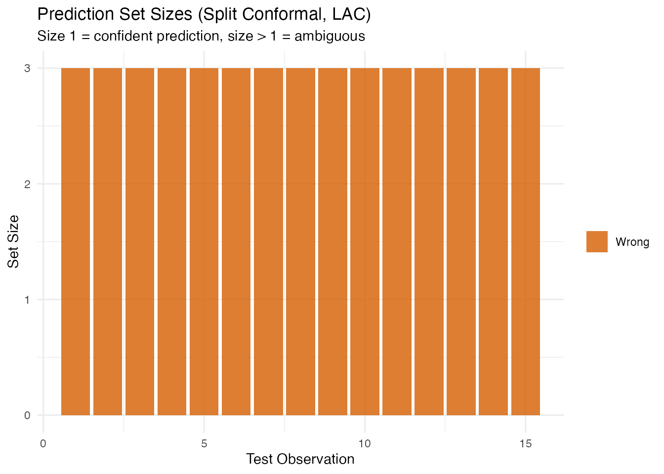

CV+ Conformal Classification

Cross-conformal (CV+) avoids the data-splitting penalty of split conformal. Each fold serves as the calibration set for the model trained on the remaining folds. All data contributes to both training and calibration.

cv_conf <- cv.conformal.classification(
  fd_train, y_train, fd_test,
  ncomp = 5, classifier = "lda",
  score.type = "lac",
  n.folds = 5,
  alpha = 0.10, seed = 42
)

cat("CV+ average set size:", round(cv_conf$average_set_size, 2), "\n")
#> CV+ average set size: 4
cat("CV+ coverage:", round(cv_conf$coverage * 100, 1), "%\n")
#> CV+ coverage: 100 %

Generic Conformal Classification

If you already have a fitted functional.logistic model, you can construct conformal prediction sets without re-fitting. Only binary classification (2 classes) is supported.

Note: Generic conformal uses in-sample calibration (the model was trained on all data including the calibration set). The coverage guarantee is broken — use this as a fast heuristic only. For valid coverage, prefer conformal.classif() or cv.conformal.classification().

# Binary classification for generic conformal (requires logistic model)
# functional.logistic expects 0/1 labels
idx_train_bin <- y_train %in% c(1, 2)
idx_test_bin <- y_test %in% c(1, 2)
train_binary <- fd_train[idx_train_bin, ]
test_binary <- fd_test[idx_test_bin, ]
y_train_bin <- as.integer(y_train[idx_train_bin] == 2)  # recode to 0/1
y_test_bin <- as.integer(y_test[idx_test_bin] == 2)

# Fit logistic model
log_model <- functional.logistic(train_binary, y_train_bin, ncomp = 3)

# Generic conformal from the fitted model
gen_conf <- conformal.generic.classification(
  log_model, train_binary, y_train_bin, test_binary,
  score.type = "lac",
  cal.fraction = 0.25, alpha = 0.10, seed = 42
)
#> Warning: conformal.generic.classification uses the pre-fitted model without
#> refitting. Calibration scores are in-sample, so coverage guarantee is broken.
#> Supply calibration.indices (held-out indices) for valid coverage, or use
#> conformal.logistic() / cv.conformal.classification() instead.

cat("Generic conformal coverage:", round(gen_conf$coverage * 100, 1), "%\n")
#> Generic conformal coverage: 100 %
cat("Average set size:", round(gen_conf$average_set_size, 2), "\n")
#> Average set size: 0.9

Comparing Classifiers

Split conformal works with different base classifiers. Compare LDA, QDA, and kNN:

classifiers <- c("lda", "qda", "knn")
results <- lapply(classifiers, function(clf) {
  res <- conformal.classif(
    fd_train, y_train, fd_test,
    ncomp = 5, classifier = clf,
    score.type = "lac",
    cal.fraction = 0.25,
    alpha = 0.10, seed = 42
  )
  data.frame(
    classifier = toupper(clf),
    coverage = res$coverage,
    avg_set_size = res$average_set_size
  )
})
df_clf <- do.call(rbind, results)
knitr::kable(df_clf, digits = 3,
             col.names = c("Classifier", "Coverage", "Avg Set Size"))

Classifier	Coverage	Avg Set Size
LDA	1	3
QDA	1	3
KNN	1	3

LAC vs APS Scoring

conf_lac <- conformal.classif(
  fd_train, y_train, fd_test,
  ncomp = 5, classifier = "lda",
  score.type = "lac",
  cal.fraction = 0.25, alpha = 0.10, seed = 42
)

conf_aps <- conformal.classif(
  fd_train, y_train, fd_test,
  ncomp = 5, classifier = "lda",
  score.type = "aps",
  cal.fraction = 0.25, alpha = 0.10, seed = 42
)

df_score <- data.frame(
  Scoring = rep(c("LAC", "APS"), each = length(y_test)),
  Set_Size = c(conf_lac$set_sizes, conf_aps$set_sizes)
)

ggplot(df_score, aes(x = .data$Scoring, y = .data$Set_Size,
                     fill = .data$Scoring)) +
  geom_boxplot(alpha = 0.7) +
  scale_fill_manual(values = c("LAC" = "#4A90D9", "APS" = "#D55E00")) +
  labs(title = "Prediction Set Size: LAC vs APS",
       subtitle = "APS produces larger sets but stronger conditional coverage",
       y = "Set Size") +
  theme(legend.position = "none")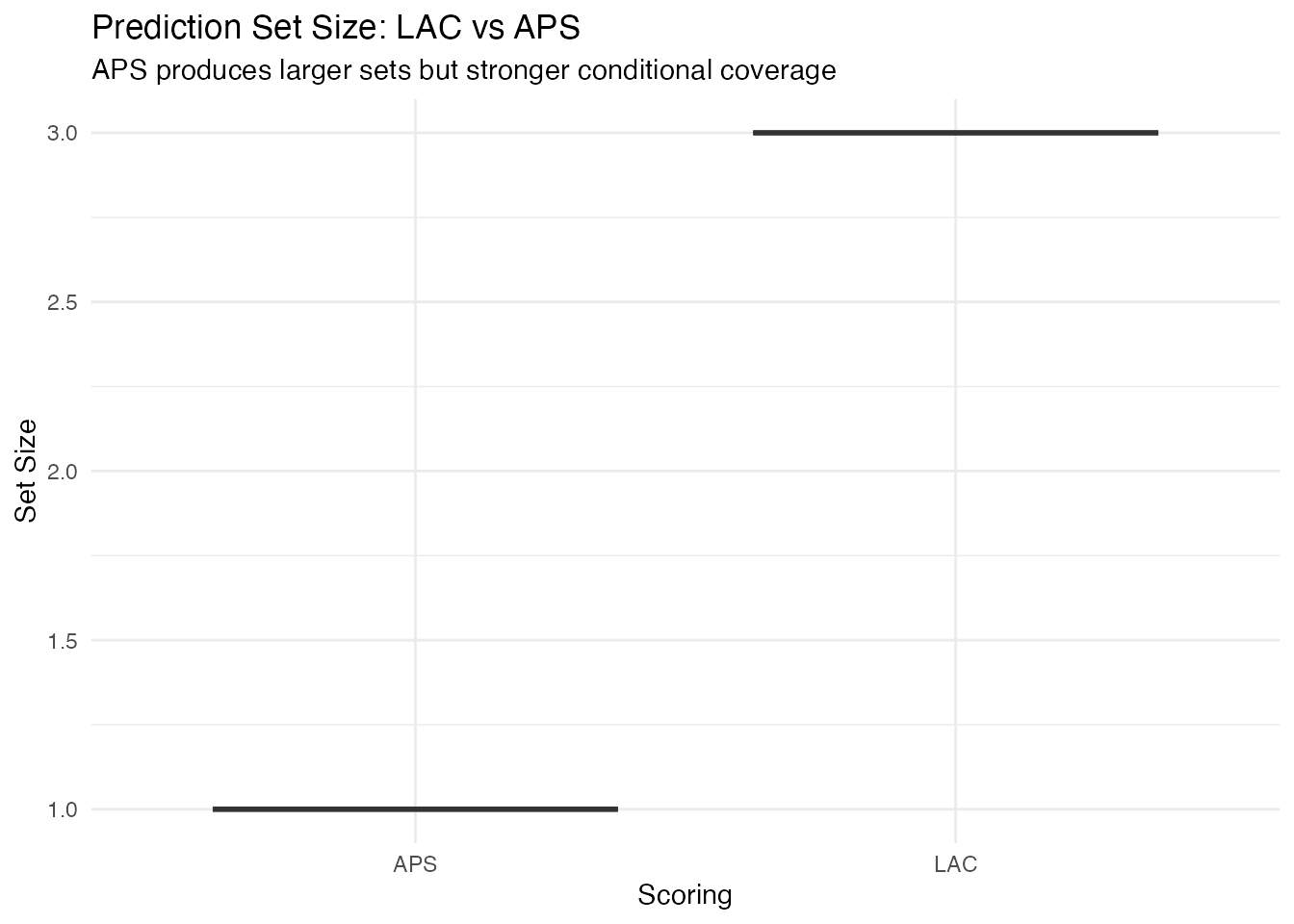

Method Comparison

Method	Function	Base models	Coverage	Sets
Split	`conformal.classif()`	LDA, QDA, kNN	$\geq 1 - \alpha$	Tightest
CV+	`cv.conformal.classification()`	LDA, QDA, kNN	$\geq 1 - 2\alpha$	Tighter (no split penalty)
Generic	`conformal.generic.classification()`	Logistic (pre-fitted, binary only)	Heuristic only	From existing model

Choosing a method:

Split conformal when data is plentiful and you want the strongest coverage guarantee ( $1 - \alpha$ ).
CV+ when data is limited and you want tighter sets — all data is used for both training and calibration.
Generic when you already have a fitted logistic model and want a quick heuristic — but note that coverage is not guaranteed (in-sample calibration).

References

Vovk, V., Gammerman, A. and Shafer, G. (2005). Algorithmic Learning in a Random World. Springer.
Sadinle, M., Lei, J. and Wasserman, L. (2019). Least ambiguous set-valued classifiers with bounded error levels. Journal of the American Statistical Association, 114(525), 223–234.
Romano, Y., Sesia, M. and Candes, E.J. (2020). Classification with valid and adaptive coverage. Advances in Neural Information Processing Systems,