Supervised Classification of Functional Data

Introduction

Supervised classification assigns functional observations to discrete groups. fdars provides seven methods:

Method	Description	Strengths
LDA	Linear discriminant analysis on FPC scores	Fast, interpretable
QDA	Quadratic discriminant analysis on FPC scores	Handles class-specific covariance
kNN	k-nearest neighbors in FPC space	Nonparametric, flexible
Kernel	Kernel classifier with functional bandwidth	Fully nonparametric
DD	Depth-vs-depth classification	Robust to outliers
Logistic	FPC-based logistic regression	Calibrated probabilities
Elastic logistic	Phase-invariant logistic	Handles misalignment

The first five methods are available through the unified fclassif() interface and support optional scalar covariates. Logistic regression uses functional.logistic(), and elastic logistic uses elastic.logistic().

Why Functional Classification?

The fundamental problem is: given a curve $X_i(t)$ , predict a class label $g_i \in \{1, \ldots, G\}$ . One might be tempted to discretize each curve at $m$ grid points and apply a standard multivariate classifier. However, this approach faces two obstacles:

Curse of dimensionality. With $m$ grid points (often 100–1000), multivariate classifiers struggle unless $n \gg m$ . Covariance matrices become singular, nearest-neighbor distances concentrate, and decision boundaries overfit.
Ignoring smoothness. Discretization treats $X_i(t_1)$ and $X_i(t_2)$ as unrelated features, discarding the continuity and smoothness of the underlying curves.

Functional classification resolves this by first projecting curves onto a low-dimensional basis — typically the leading FPC directions — and then classifying in that reduced space. This simultaneously regularizes the problem (since $K \ll m$ ) and respects the functional structure (since FPCs capture the dominant modes of variation).

For methods that work directly in function space (kernel classifier, DD classifier), distances are computed using proper functional metrics ( $L^2$ norm or depth), avoiding discretization artifacts entirely.

Mathematical Framework

All FPC-based methods (LDA, QDA, kNN) start by computing the scores $\boldsymbol\xi_i = (\xi_{i1}, \ldots, \xi_{iK})^T$ where $\xi_{ik} = \int [X_i(t) - \bar{X}(t)]\phi_k(t)\,dt$ and $\phi_k$ are the eigenfunctions of the pooled covariance operator. Classification then operates in $\mathbb{R}^K$ .

Linear Discriminant Analysis (LDA)

LDA assumes that the FPC scores within each class are Gaussian with a common covariance:

$\boldsymbol\xi \mid g = k \;\sim\; \mathcal{N}(\boldsymbol\mu_k,\, \boldsymbol\Sigma_{\text{pool}})$

The pooled covariance is:

$\hat{\boldsymbol\Sigma}_{\text{pool}} = \frac{1}{n - G}\sum_{g=1}^G \sum_{i \in g}(\boldsymbol\xi_i - \bar{\boldsymbol\xi}_g)(\boldsymbol\xi_i - \bar{\boldsymbol\xi}_g)^T$

Classification uses the log-posterior discriminant:

$\delta_g(\boldsymbol\xi) = \log\pi_g - \tfrac{1}{2}(\boldsymbol\xi - \boldsymbol\mu_g)^T \boldsymbol\Sigma_{\text{pool}}^{-1}(\boldsymbol\xi - \boldsymbol\mu_g)$

where $\pi_g$ is the prior probability of class $g$ (estimated by class proportions). The observation is assigned to $\hat{g} = \arg\max_g \delta_g(\boldsymbol\xi)$ . Because $\boldsymbol\Sigma_{\text{pool}}$ is shared, the decision boundaries are linear (hyperplanes) in the FPC score space.

Quadratic Discriminant Analysis (QDA)

QDA relaxes the equal-covariance assumption by estimating a class-specific covariance $\boldsymbol\Sigma_g$ for each group. The discriminant becomes:

$\delta_g(\boldsymbol\xi) = \log\pi_g - \tfrac{1}{2}\log|\boldsymbol\Sigma_g| - \tfrac{1}{2}(\boldsymbol\xi - \boldsymbol\mu_g)^T\boldsymbol\Sigma_g^{-1}(\boldsymbol\xi - \boldsymbol\mu_g)$

The additional $\log|\boldsymbol\Sigma_g|$ term penalizes classes with large spread. Decision boundaries are now quadratic (ellipsoidal). QDA is more flexible than LDA but requires enough observations per class to reliably estimate $\boldsymbol\Sigma_g$ — roughly $n_g > K(K+1)/2$ as a rule of thumb.

k-Nearest Neighbors (kNN)

kNN classifies by majority vote among the $k$ closest training curves in FPC space, using Euclidean distance:

$d(\boldsymbol\xi_i, \boldsymbol\xi_j) = \|\boldsymbol\xi_i - \boldsymbol\xi_j\|_2 = \sqrt{\sum_{l=1}^K (\xi_{il} - \xi_{jl})^2}$

The predicted class is whichever label appears most often among the $k$ neighbors. kNN makes no distributional assumptions, making it robust to non-Gaussian score distributions and nonlinear class boundaries. The choice of $k$ is typically made via cross-validation: small $k$ gives flexible but noisy boundaries; large $k$ gives smoother but potentially biased boundaries.

Kernel Classifier

The kernel classifier works directly in function space without dimension reduction. It uses the $L^2$ functional distance with Simpson’s rule integration weights:

$d(X_i, X_j) = \sqrt{\int_0^1 [X_i(t) - X_j(t)]^2\,dt}$

Classification uses a Gaussian kernel to weight contributions from training curves:

$K(d, h) = \exp\!\left(-\frac{d^2}{2h^2}\right)$

The predicted class is:

$\hat{g}(X) = \arg\max_g \sum_{j:\,y_j = g} K\bigl(d(X, X_j),\, h\bigr)$

That is, for each class, the kernel weights of all training curves in that class are summed, and the class with the largest total weight wins. The bandwidth $h$ controls the locality of the classifier. fclassif() selects $h$ via leave-one-out cross-validation over a grid of distance percentiles.

DD-Classifier (Depth-vs-Depth)

The depth-based classifier avoids both dimension reduction and distance computation. Instead, it computes the statistical depth of each curve with respect to each class distribution:

$D_g(X_i) = \text{depth of } X_i \text{ w.r.t. class } g$

using the Fraiman–Muniz integrated depth:

$D_{\text{FM}}(X) = \int_0^1 D_1\bigl(X(t);\, F_t\bigr)\,dt$

where $D_1$ is the univariate depth (one minus twice the distance from the median CDF value) and $F_t$ is the marginal distribution at time $t$ .

For $G$ classes, each curve is mapped to a point $(D_1(X_i), \ldots, D_G(X_i)) \in \mathbb{R}^G$ and classification proceeds in this “depth-depth” space. The simplest rule assigns to $\hat{g} = \arg\max_g D_g(X_i)$ : the class in which the curve is most “central”. This approach is robust to outliers because depth is a rank-based measure.

Iris as Functional Data

Instead of a toy simulation we use the classic iris dataset, transformed into functional data via the Andrews transformation. This maps each 4-dimensional observation to a curve on $[-\pi, \pi]$ using a Fourier expansion — preserving Euclidean distances up to a constant factor.

The three species (setosa, versicolor, virginica) are the classes. Crucially, versicolor and virginica overlap substantially, making this a non-trivial classification task.

andrews_transform <- function(X, m = 200) {
  if (is.data.frame(X)) X <- as.matrix(X)
  n <- nrow(X)
  p <- ncol(X)
  t_grid <- seq(-pi, pi, length.out = m)

  basis <- matrix(0, m, p)
  basis[, 1] <- 1 / sqrt(2)
  for (j in 2:p) {
    k <- ceiling((j - 1) / 2)
    if (j %% 2 == 0) {
      basis[, j] <- sin(k * t_grid)
    } else {
      basis[, j] <- cos(k * t_grid)
    }
  }

  fdata(X %*% t(basis), argvals = t_grid)
}

X_raw <- as.matrix(iris[, 1:4])
X <- scale(X_raw)
species <- iris$Species
y <- as.integer(species)  # 1 = setosa, 2 = versicolor, 3 = virginica

fd <- andrews_transform(X)

plot(fd, color = species, alpha = 0.35, show.mean = TRUE,
     palette = c("setosa" = "#E69F00", "versicolor" = "#56B4E9",
                 "virginica" = "#009E73")) +
  labs(x = expression(t), y = expression(f[x](t)),
       title = "Iris Andrews Curves by Species")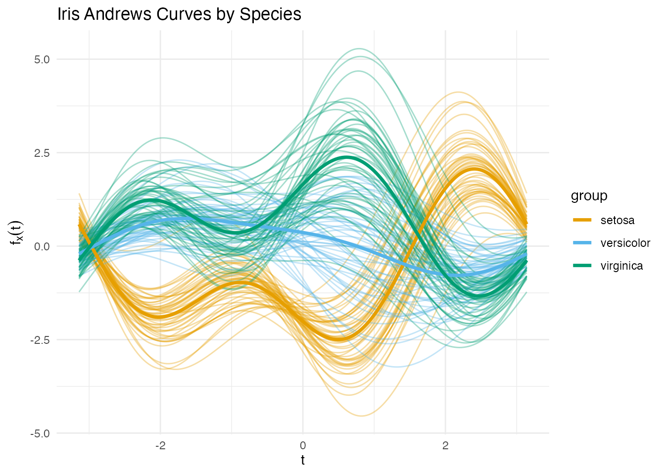

Setosa is well separated, but versicolor and virginica overlap — exactly the kind of challenge where classifier choice matters.

Comparing All Five Methods

methods <- c("lda", "qda", "knn", "kernel", "dd")
results <- list()

for (meth in methods) {
  if (meth == "knn") {
    results[[meth]] <- fclassif(fd, y, method = meth, ncomp = 3, k = 7)
  } else {
    results[[meth]] <- fclassif(fd, y, method = meth, ncomp = 3)
  }
}

acc_df <- data.frame(
  Method = toupper(methods),
  Training_Accuracy = sapply(results, function(r) round(r$accuracy, 3))
)
print(acc_df)
#>        Method Training_Accuracy
#> lda       LDA             0.973
#> qda       QDA             0.973
#> knn       KNN             0.960
#> kernel KERNEL             0.960
#> dd         DD             0.840

Training accuracy alone can be misleading — QDA and kNN may overfit. Cross-validation gives a fairer picture (see below).

Confusion Matrix

The LDA confusion matrix reveals where errors concentrate:

plot(results[["lda"]])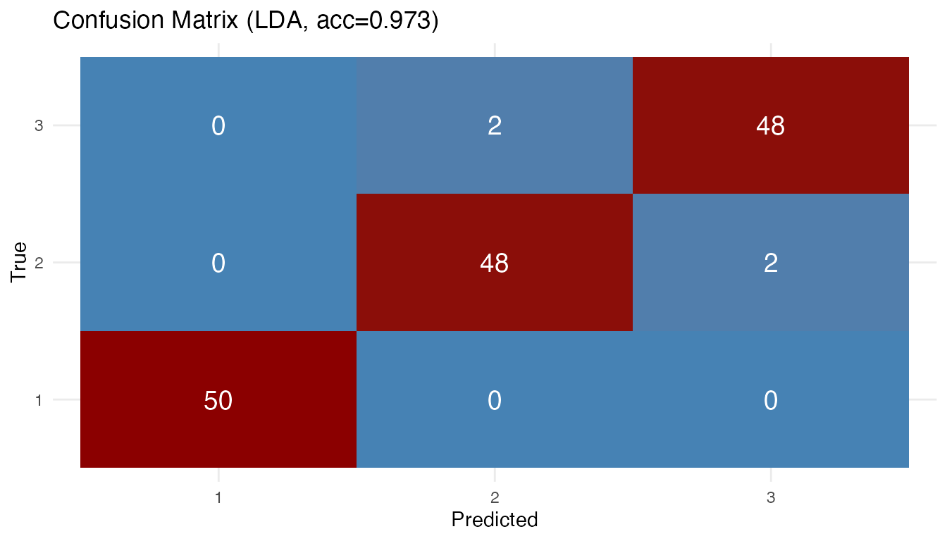

Most errors are between versicolor and virginica, as expected from the overlapping Andrews curves. Setosa is perfectly classified because its curves are well separated in the FPC score space.

Cross-Validation

fclassif.cv() evaluates out-of-sample error via k-fold cross-validation. This gives the most honest estimate of how each classifier would perform on new data, guarding against the optimism of training accuracy.

set.seed(42)
cv_results <- list()
for (meth in methods) {
  cv_results[[meth]] <- fclassif.cv(fd, y, method = meth,
                                     ncomp = 3, nfold = 10, seed = 42)
}

cv_df <- data.frame(
  Method = toupper(methods),
  CV_Error = sapply(cv_results, function(r) round(r$error.rate, 3)),
  CV_Accuracy = sapply(cv_results, function(r) round(1 - r$error.rate, 3))
)
print(cv_df)
#>        Method CV_Error CV_Accuracy
#> lda       LDA    0.027       0.973
#> qda       QDA    0.033       0.967
#> knn       KNN    0.040       0.960
#> kernel KERNEL    1.000       0.000
#> dd         DD    1.000       0.000

The CV error rates account for overfitting. Methods that had perfect training accuracy (like QDA) may show higher CV error than simpler methods (like LDA), especially when sample sizes per class are small relative to the number of parameters.

Choosing the Number of Components

Cross-validation can also help select the optimal number of FPC components. Too few loses discriminative information; too many introduces noise.

ncomp_range <- 1:6
cv_by_ncomp <- sapply(ncomp_range, function(k) {
  fclassif.cv(fd, y, method = "lda", ncomp = k, nfold = 10, seed = 42)$error.rate
})

df_ncomp <- data.frame(ncomp = ncomp_range, error = cv_by_ncomp)
ggplot(df_ncomp, aes(x = ncomp, y = error)) +
  geom_line() +
  geom_point(size = 2) +
  labs(x = "Number of FPC Components", y = "10-Fold CV Error Rate",
       title = "LDA on Iris: Component Selection") +
  scale_x_continuous(breaks = ncomp_range)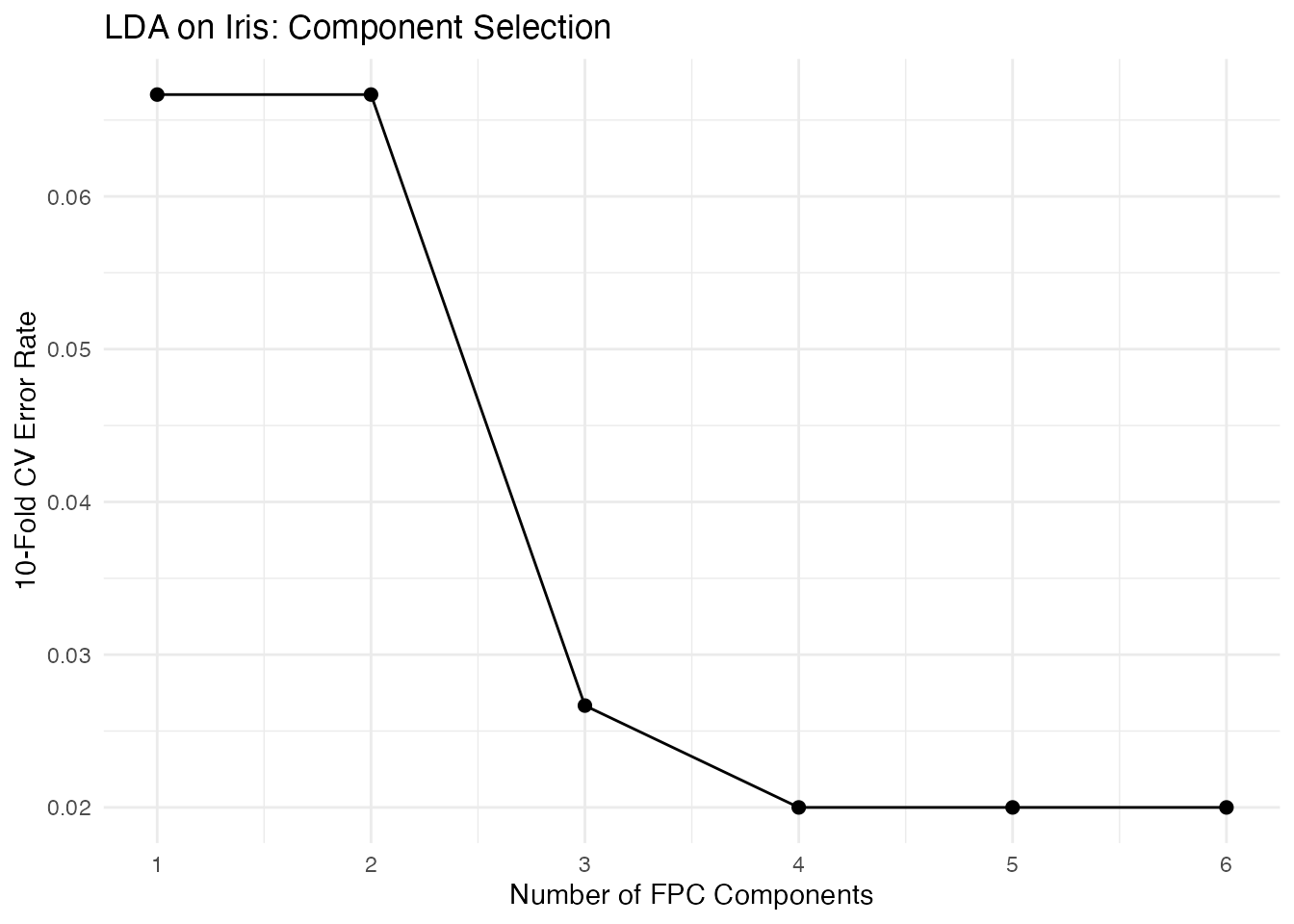

The optimal number of components balances two effects: adding early components captures the dominant modes of between-class variation, improving discrimination. Adding later components brings in directions that are mainly within-class noise, diluting the signal.

Functional Logistic Regression

For binary classification, functional.logistic() fits a logistic regression model using FPC scores as features. Unlike the discriminative methods above, this produces calibrated probabilities — useful when you need confidence in the classification, not just a label.

The IRLS Algorithm

The functional logistic model uses the logit link on FPC scores:

$\log\frac{P(Y_i = 1)}{1 - P(Y_i = 1)} = \alpha + \sum_{k=1}^K \gamma_k \xi_{ik}$

This is estimated via Iteratively Reweighted Least Squares (IRLS), which alternates between:

Working response: $z_i = \hat\eta_i + (y_i - \hat{p}_i) / [\hat{p}_i(1 - \hat{p}_i)]$
Working weights: $w_i = \hat{p}_i(1 - \hat{p}_i)$
Weighted least squares: update $\hat\gamma$ by regressing $z$ on $\Xi$ with weights $w$

Convergence is monitored via the log-likelihood:

$\ell(\gamma) = \sum_{i=1}^n \bigl[y_i \log p_i + (1 - y_i)\log(1 - p_i)\bigr]$

Binary Classification Example

# Create binary response from iris species (setosa vs rest)
y_bin <- as.numeric(y == 1)  # 1 = setosa, 0 = versicolor/virginica

logit_fit <- functional.logistic(fd, y_bin, ncomp = 3)
print(logit_fit)
#> Functional Logistic Regression
#> ==============================
#>   Number of observations: 150 
#>   Number of FPC components: 3 
#>   Accuracy: 1 
#>   Log-likelihood: 0 
#>   Iterations: 100

cat("Probabilities range:", range(logit_fit$probabilities), "\n")
#> Probabilities range: 2.218142e-45 1

Estimated probabilities near 0 or 1 indicate confident classification; values near 0.5 indicate curves in the overlap region where the predictor’s FPC scores do not clearly separate the two classes.

Probability Interpretation

Unlike discriminant methods (LDA/QDA), functional logistic regression directly models $P(Y = 1 | X)$ . This makes it natural for:

Risk scoring: rank observations by predicted probability
Threshold tuning: adjust the decision boundary beyond 0.5
Calibration: the predicted probabilities approximate true class frequencies

Elastic Logistic Regression

When curves exhibit phase variability (timing differences), standard logistic regression on FPC scores may confound amplitude and phase effects. elastic.logistic() jointly estimates alignment warping functions and logistic regression coefficients in the SRSF domain.

See vignette("articles/elastic-regression") for the full elastic regression framework, including elastic.logistic() and elastic.pcr().

Choosing a Classifier

The table below summarizes practical considerations:

Criterion	LDA	QDA	kNN	Kernel	DD	Logistic
Assumptions	Common cov.	Class-specific cov.	None	None	None	Linear in FPC space
Min. $n_g$	$> K$	$> K(K+1)/2$	$> k$	$> 20$	$> 20$	$> K$
Boundaries	Linear	Quadratic	Flexible	Flexible	Depth-based	Linear
Tuning	$K$ only	$K$ only	$K$ , $k$	$h$	$K$	$K$
Speed	Fast	Fast	Moderate	Slow	Moderate	Fast
Robustness	Low	Low	Moderate	Moderate	High	Low
Probabilities	Posterior	Posterior	No	No	No	Calibrated

Rules of thumb:

Start with LDA as a baseline — it is fast, interpretable, and often competitive.
Try QDA when you suspect classes have different shapes in FPC space (different covariance patterns).
Use kNN when decision boundaries may be nonlinear and you have enough data per class.
Use the kernel classifier for small-to-moderate datasets where you want to avoid the FPC projection step entirely.
Use DD when robustness to outliers is paramount or distributional assumptions are suspect.
Use logistic regression when you need calibrated probabilities or want to interpret coefficients as log-odds.

References

Delaigle, A. and Hall, P. (2012). Achieving near perfect classification for functional data. Journal of the Royal Statistical Society: Series B, 74(2), 267–286.
Cuevas, A., Febrero, M., and Fraiman, R. (2007). Robust estimation and classification for functional data via projection pursuit. Computational Statistics, 22(3), 481–496.
Li, J. and Yu, T. (2008). DD-classifier: nonparametric classification procedure based on DD-plot. Journal of the American Statistical Association, 103(483), 737–747.
Lopez-Pintado, S. and Romo, J. (2009). On the concept of depth for functional data. Journal of the American Statistical Association, 104(486), 718–734.