Cross-Validation: Honest Model Comparison with OOF Predictions

The individual *.cv functions (fregre.pc.cv, fregre.basis.cv, fregre.np.cv) tune hyperparameters but don’t produce out-of-fold (OOF) predictions — predictions where each observation is predicted exactly once, when it sits in the held-out fold. OOF predictions give an honest estimate of generalisation performance and are the standard output of a cross-validation workflow.

cv.fdata() provides a unified framework that wraps any fit/predict workflow and returns OOF predictions for the entire dataset.

Step	What It Does	Outcome
Data preparation	Load 215 Tecator NIR spectra with fat response	`fdata` object ready for regression
Basic CV	5-fold CV with fixed hyperparameters	OOF predictions + RMSE/MAE/R2
Nested CV	Outer 5-fold, inner CV selects ncomp per fold	Unbiased evaluation with automatic tuning
Method comparison	Run seven methods on identical fold splits	Fair head-to-head comparison table
Visualisation	Observed vs predicted + per-fold residual boxplots	Diagnose prediction quality across folds

Key result: Nested CV avoids the optimistic bias of evaluating on the same data used to select hyperparameters, giving realistic out-of-sample error estimates.

Tecator Data

The Tecator dataset contains 215 meat samples, each with an absorbance spectrum measured at 100 wavelengths (850–1050 nm) and laboratory-measured fat content. This is the same dataset used in the Tecator regression example.

data(tecator, package = "fda.usc")

absorp_data <- tecator$absorp.fdata$data
wavelengths <- as.numeric(tecator$absorp.fdata$argvals)
fd <- fdata(absorp_data, argvals = wavelengths)
fat <- tecator$y$Fat
n <- nrow(fd$data)

cat("Samples:", n, "\n")
#> Samples: 215
cat("Wavelengths:", ncol(fd$data), "(", range(wavelengths), "nm)\n")
#> Wavelengths: 100 ( 850 1050 nm)
cat("Fat range:", round(range(fat), 1), "%\n")
#> Fat range: 0.9 49.1 %

plot(fd) +
  labs(title = "NIR Absorbance Spectra (215 meat samples)",
       x = "Wavelength (nm)", y = "Absorbance")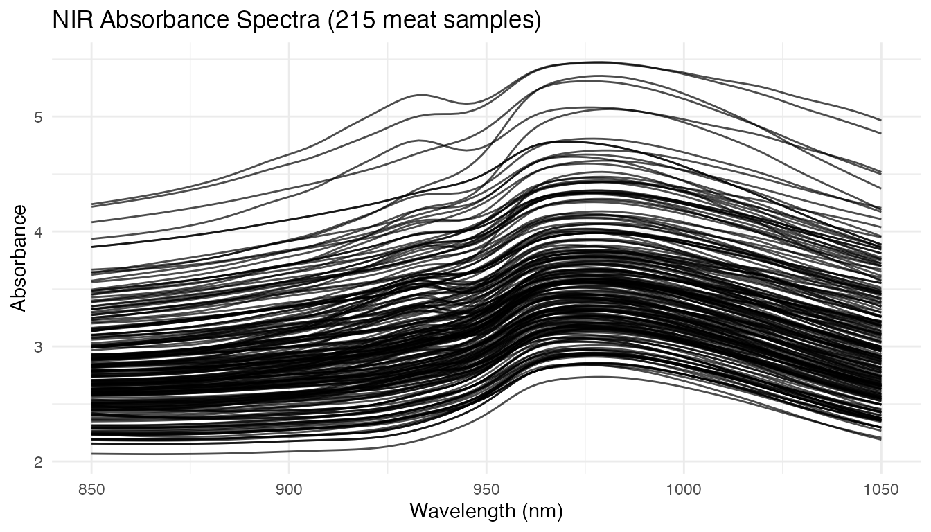

Pre-Processing

Raw absorbance spectra contain baseline shifts. Smoothing with B-splines and taking the second derivative removes these effects and enhances spectral features — we’ll use both representations for cross-validation.

coefs_raw <- fdata2basis(fd, nbasis = 30, type = "bspline")
fd_smooth <- basis2fdata(coefs_raw, wavelengths)

fd_deriv2 <- deriv(deriv(fd_smooth))

Basic K-Fold Cross-Validation

Pass any fitting function to cv.fdata and it handles the fold loop. Every observation is predicted exactly once:

cv_result <- cv.fdata(fd_smooth, fat,
  fit.fn = function(fd, y, ...) fregre.pc(fd, y, ncomp = 6),
  kfold = 5, seed = 42)
print(cv_result)
#> K-Fold Cross-Validation (cv.fdata)
#>   Type: regression 
#>   Folds: 5 
#>   Observations: 215  
#> 
#> Overall metrics:
#>   RMSE: 3.164 
#>   MAE:  2.466 
#>   R2:   0.938 
#> 
#> Per-fold RMSE range: [2.785, 3.681]

cat("OOF predictions:", length(cv_result$oof.predictions), "\n")
#> OOF predictions: 215
cat("Any missing:", any(is.na(cv_result$oof.predictions)), "\n")
#> Any missing: FALSE

Nested Cross-Validation

When hyperparameters are tuned, evaluating on the same data used for selection gives an optimistically biased error estimate. Nested CV fixes this: the outer folds produce OOF predictions while an inner CV selects optimal parameters on each training fold independently.

cv_nested <- cv.fdata(fd_smooth, fat,
  fit.fn = function(fd, y, ...) {
    cv_inner <- fregre.pc.cv(fd, y, ncomp.range = 1:15, kfold = 5)
    cv_inner$model
  },
  kfold = 5, seed = 42)
print(cv_nested)
#> K-Fold Cross-Validation (cv.fdata)
#>   Type: regression 
#>   Folds: 5 
#>   Observations: 215  
#> 
#> Overall metrics:
#>   RMSE: 2.646 
#>   MAE:  2 
#>   R2:   0.9567 
#> 
#> Per-fold RMSE range: [2.197, 3.175]

Inspect which ncomp was selected in each outer fold — different training subsets may favour different complexities:

ncomps <- sapply(cv_nested$fold.models, function(m) m$ncomp)
cat("ncomp per fold:", ncomps, "\n")
#> ncomp per fold: 15 15 15 15 15

Comparing Methods on Identical Folds

Because cv.fdata accepts any fit.fn, you can fairly compare methods by using the same seed (which fixes the fold assignments):

# Absorbance-based methods
cv_pc <- cv.fdata(fd_smooth, fat,
  fit.fn = function(fd, y, ...) fregre.pc(fd, y, ncomp = 6),
  kfold = 5, seed = 42)

cv_basis <- cv.fdata(fd_smooth, fat,
  fit.fn = function(fd, y, ...) {
    cv_inner <- fregre.basis.cv(fd, y,
      lambda.range = c(0.001, 0.01, 0.1, 1, 10))
    fregre.basis(fd, y, lambda = cv_inner$optimal.lambda)
  },
  kfold = 5, seed = 42)

cv_lm <- cv.fdata(fd_smooth, fat,
  fit.fn = function(fd, y, ...) {
    cv_inner <- fregre.lm.cv(fd, y, k.range = 1:15, nfold = 5)
    fregre.lm(fd, y, ncomp = cv_inner$optimal.k)
  },
  kfold = 5, seed = 42)

cv_knn <- cv.fdata(fd_smooth, fat,
  fit.fn = function(fd, y, ...) fregre.np(fd, y, type.S = "kNN.gCV"),
  kfold = 5, seed = 42)

# Second-derivative methods
cv_pc_d2 <- cv.fdata(fd_deriv2, fat,
  fit.fn = function(fd, y, ...) {
    cv_inner <- fregre.pc.cv(fd, y, ncomp.range = 1:15, kfold = 5)
    cv_inner$model
  },
  kfold = 5, seed = 42)

cv_lm_d2 <- cv.fdata(fd_deriv2, fat,
  fit.fn = function(fd, y, ...) {
    cv_inner <- fregre.lm.cv(fd, y, k.range = 1:15, nfold = 5)
    fregre.lm(fd, y, ncomp = cv_inner$optimal.k)
  },
  kfold = 5, seed = 42)

cv_knn_elastic <- cv.fdata(fd_deriv2, fat,
  fit.fn = function(fd, y, ...) fregre.np(fd, y, type.S = "kNN.gCV",
                                           metric = metric.elastic),
  kfold = 5, seed = 42)

comparison <- data.frame(
  Method = c("PC (absorbance)", "Basis (absorbance)",
             "fregre.lm (absorbance)", "k-NN / L2 (absorbance)",
             "PC (2nd derivative)", "fregre.lm (2nd derivative)",
             "k-NN / elastic (2nd derivative)"),
  RMSE = round(c(cv_pc$metrics$RMSE, cv_basis$metrics$RMSE,
                  cv_lm$metrics$RMSE, cv_knn$metrics$RMSE,
                  cv_pc_d2$metrics$RMSE, cv_lm_d2$metrics$RMSE,
                  cv_knn_elastic$metrics$RMSE), 3),
  MAE = round(c(cv_pc$metrics$MAE, cv_basis$metrics$MAE,
                 cv_lm$metrics$MAE, cv_knn$metrics$MAE,
                 cv_pc_d2$metrics$MAE, cv_lm_d2$metrics$MAE,
                 cv_knn_elastic$metrics$MAE), 3),
  R2 = round(c(cv_pc$metrics$R2, cv_basis$metrics$R2,
                cv_lm$metrics$R2, cv_knn$metrics$R2,
                cv_pc_d2$metrics$R2, cv_lm_d2$metrics$R2,
                cv_knn_elastic$metrics$R2), 3)
)
knitr::kable(comparison, caption = "5-fold OOF performance (same folds)")

5-fold OOF performance (same folds)
Method	RMSE	MAE	R2
PC (absorbance)	3.164	2.466	0.938
Basis (absorbance)	2.898	2.234	0.948
fregre.lm (absorbance)	10390.709	7114.562	-668275.125
k-NN / L2 (absorbance)	8.011	5.967	0.603
PC (2nd derivative)	2.374	1.808	0.965
fregre.lm (2nd derivative)	1234.593	1016.676	-9433.377
k-NN / elastic (2nd derivative)	1.737	1.178	0.981

Visualising OOF Predictions

Observed vs predicted and per-fold residual boxplots for the nested CV result:

valid <- !is.na(cv_nested$oof.predictions)
df_pred <- data.frame(
  Observed = fat[valid],
  Predicted = cv_nested$oof.predictions[valid],
  Fold = factor(cv_nested$folds[valid]),
  Residual = fat[valid] - cv_nested$oof.predictions[valid]
)

p1 <- ggplot(df_pred, aes(x = Observed, y = Predicted)) +
  geom_point(colour = "steelblue", alpha = 0.6) +
  geom_abline(intercept = 0, slope = 1, linetype = "dashed", colour = "red") +
  labs(title = "Nested CV: Observed vs Predicted",
       x = "Observed fat (%)", y = "Predicted fat (%)")

p2 <- ggplot(df_pred, aes(x = Fold, y = Residual)) +
  geom_boxplot(fill = "lightblue", alpha = 0.7) +
  geom_hline(yintercept = 0, linetype = "dashed", colour = "red") +
  labs(title = "Per-Fold Residuals", x = "Fold", y = "Residual")

library(patchwork)
p1 + p2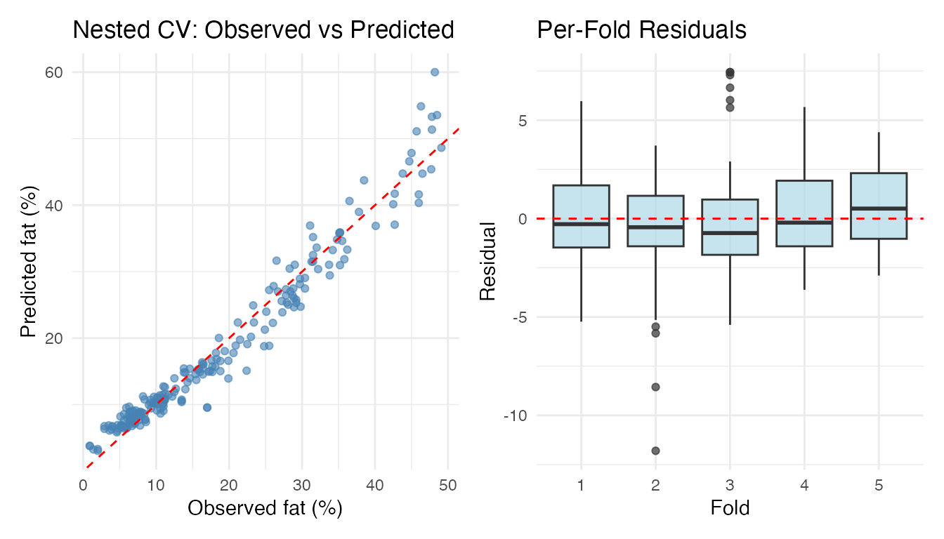

Comparing OOF Predictions Across Methods

method_levels <- c("PC (absorbance)", "Basis (absorbance)",
                   "fregre.lm (absorbance)", "k-NN / L2 (absorbance)",
                   "PC (2nd deriv)", "fregre.lm (2nd deriv)",
                   "k-NN / elastic (2nd deriv)")

df_oof <- data.frame(
  Observed = rep(fat, 7),
  Predicted = c(cv_pc$oof.predictions, cv_basis$oof.predictions,
                cv_lm$oof.predictions, cv_knn$oof.predictions,
                cv_pc_d2$oof.predictions, cv_lm_d2$oof.predictions,
                cv_knn_elastic$oof.predictions),
  Method = factor(rep(method_levels, each = n), levels = method_levels)
)

ggplot(df_oof, aes(x = Observed, y = Predicted)) +
  geom_point(alpha = 0.5, colour = "#0072B2") +
  geom_abline(intercept = 0, slope = 1, linetype = "dashed", colour = "red") +
  facet_wrap(~ Method, ncol = 2) +
  labs(title = "Out-of-Fold Predictions by Method",
       x = "Observed fat (%)", y = "OOF predicted fat (%)")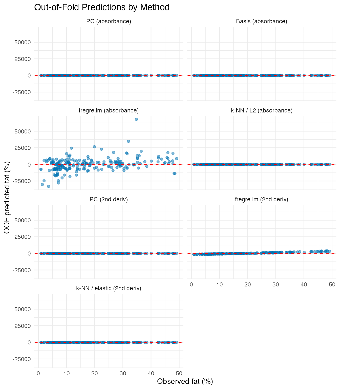

Per-Fold Stability

The fold.metrics data frame shows how performance varies across folds — large variation can indicate sensitivity to the particular train/test split:

knitr::kable(cv_nested$fold.metrics, digits = 3,
             caption = "Per-fold metrics (nested CV)")

Per-fold metrics (nested CV)
fold	n	RMSE	MAE	R2
1	45	2.368	1.866	0.966
2	44	3.012	2.055	0.945
3	44	3.175	2.401	0.940
4	41	2.273	1.828	0.967
5	41	2.197	1.828	0.969

Stratified Folds

By default, cv.fdata uses stratified fold assignment: the response is binned into quantile groups and observations are sampled within each bin. This ensures every fold has a similar distribution of fat content, which matters because the Tecator dataset has a right-skewed fat distribution.

folds_strat <- fdars::: .create_folds(fat, kfold = 5, type = "regression",
                                       stratified = TRUE, seed = 1)
folds_rand <- fdars::: .create_folds(fat, kfold = 5, type = "regression",
                                      stratified = FALSE, seed = 1)

df_folds <- data.frame(
  Fat = rep(fat, 2),
  Fold = factor(c(folds_strat, folds_rand)),
  Type = rep(c("Stratified", "Random"), each = n)
)

ggplot(df_folds, aes(x = Fold, y = Fat)) +
  geom_boxplot(fill = "lightblue", alpha = 0.7) +
  facet_wrap(~ Type) +
  labs(title = "Fat Distribution Across Folds",
       y = "Fat (%)")

Set stratified = FALSE to use purely random assignment (matching the existing *.cv functions).

Custom Predict Functions

Some models need a custom prediction step. The predict.fn argument receives the fitted model and new data, and returns predictions:

cv_custom <- cv.fdata(fd_smooth, fat,
  fit.fn = function(fd, y, ...) fregre.basis(fd, y, nbasis = 20, lambda = 0.1),
  predict.fn = function(model, newdata) predict(model, newdata),
  kfold = 5, seed = 42)
cat("Custom predict RMSE:", round(cv_custom$metrics$RMSE, 3), "\n")
#> Custom predict RMSE: 3.337

Summary

Feature	`*.cv` functions	`cv.fdata`
Hyperparameter tuning	Yes (internal)	Via `fit.fn` wrapper
OOF predictions	No	Yes (full dataset)
Stratified folds	No	Yes (default)
Method-agnostic	No (one per method)	Yes (any fit/predict)
Nested CV	No	Yes (compose with `*.cv`)
Per-fold models	No	Yes (`$fold.models`)
Per-fold metrics	No	Yes (`$fold.metrics`)