Regression Diagnostics

Overview

After fitting a functional regression model, it is essential to check whether the assumptions hold, whether any observations unduly influence the fit, and whether the results are stable. The fdars package provides seven diagnostic tools adapted for FPC-based functional regression.

Regression Diagnostics: 6 panels showing influence, DFBETAS, importance, depth, residuals, VIF

Supported Models

Method	Function	`fregre.lm`	`functional.logistic`
Influence (leverage, Cook’s D)	`fregre.influence`	yes
DFBETAS / DFFITS	`fregre.dfbetas`	yes
VIF	`fregre.vif`	yes	yes
Permutation importance	`fregre.importance`	yes	yes
Conditional importance	`fregre.conditional.importance`	yes	yes
Regression depth	`fregre.depth`	yes	yes
Explanation stability	`fregre.stability`	model-free	model-free

Why only fregre.lm and functional.logistic? All diagnostic functions operate on the FPC scores and regression coefficients produced by fregre.lm() or functional.logistic(). Other model types (fregre.pc, fregre.np, fregre.basis) use different internal structures and are not currently supported by the Rust diagnostics backend.

Why not nonparametric models? Nonparametric models like fregre.np() (kernel regression) and KNN do not produce coefficients or an explicit hat matrix, so leverage, Cook’s distance, DFBETAS, VIF, and beta decomposition are undefined. Permutation importance could in principle work for any model, but the current implementation requires the FPC score representation from fregre.lm.

Setup

Simulated Data

We simulate functional data with a known coefficient function. In applied terms, think of a manufacturing process where sensor curves predict a quality measure — diagnostics help identify faulty sensors (influential observations) and unstable model regions.

n <- 80
m <- 100
t_grid <- seq(0, 1, length.out = m)

beta_true <- 2 * dnorm(t_grid, 0.3, 0.08) - 1.5 * dnorm(t_grid, 0.7, 0.08)
beta_true <- beta_true / max(abs(beta_true))

X <- matrix(0, n, m)
for (i in 1:n) {
  X[i, ] <- sin(2 * pi * t_grid) + 0.5 * rnorm(1) * cos(4 * pi * t_grid) +
            rnorm(m, sd = 0.1)
}

dt <- t_grid[2] - t_grid[1]
y <- numeric(n)
for (i in 1:n) {
  y[i] <- sum(beta_true * X[i, ]) * dt + rnorm(1, sd = 0.3)
}

fdataobj <- fdata(X, argvals = t_grid)
model <- fregre.lm(fdataobj, y, ncomp = 5)

Influence and Case Deletion

These methods identify observations that disproportionately affect the fitted model. Removing a single influential observation can substantially change the coefficients, fitted values, and predictions.

Supported models: fregre.lm only. These methods require the hat matrix, which is only defined for linear models.

Influence diagnostics: leverage, Cook's D, DFBETAS, VIF

Leverage and Cook’s Distance

In plain English: Leverage measures how far an observation’s FPC scores are from the centre of the score space — think of it as “how unusual is this curve’s shape?” Cook’s distance combines leverage with residual size to measure the overall influence on the model. A point with high leverage and a large residual is influential: removing it would noticeably change the regression coefficients.

Mathematically: In the FPC regression $\hat{\boldsymbol{y}} = \boldsymbol{H}\boldsymbol{y}$ , the hat matrix is

$\boldsymbol{H} = \boldsymbol{\Xi}(\boldsymbol{\Xi}^\top\boldsymbol{\Xi})^{-1}\boldsymbol{\Xi}^\top,$

where $\boldsymbol{\Xi}$ is the $n \times (K+1)$ augmented score matrix. The diagonal $h_{ii}$ is the leverage of observation $i$ . Observations with $h_{ii} > 2(K+1)/n$ are flagged as high-leverage.

Cook’s distance combines leverage and residual:

$D_i = \frac{e_i^2}{(K+1)\,\hat{\sigma}^2} \cdot \frac{h_{ii}}{(1-h_{ii})^2}.$

The classic threshold is $D_i > 4/n$ . A high Cook’s $D$ means the observation pulls the fitted surface toward itself.

influence <- fregre.influence(model, data = fdataobj)

df_inf <- data.frame(
  Observation = 1:n,
  Leverage = influence$leverage,
  CooksD = influence$cooks_distance
)

ggplot(df_inf, aes(x = .data$Leverage, y = .data$CooksD)) +
  geom_point(color = "#7B2D8E", size = 2, alpha = 0.7) +
  geom_text(data = subset(df_inf, CooksD > quantile(CooksD, 0.95)),
            aes(label = .data$Observation), hjust = -0.3, size = 3,
            color = "#D55E00") +
  geom_hline(yintercept = 4 / n, linetype = "dashed",
             color = "#D55E00", alpha = 0.5) +
  annotate("text", x = max(df_inf$Leverage) * 0.9, y = 4 / n + 0.001,
           label = "4/n threshold", color = "#D55E00", size = 3) +
  labs(title = "Influence Diagnostics",
       subtitle = "High leverage + high Cook's D = influential observations",
       x = "Leverage (Hat value)", y = "Cook's Distance")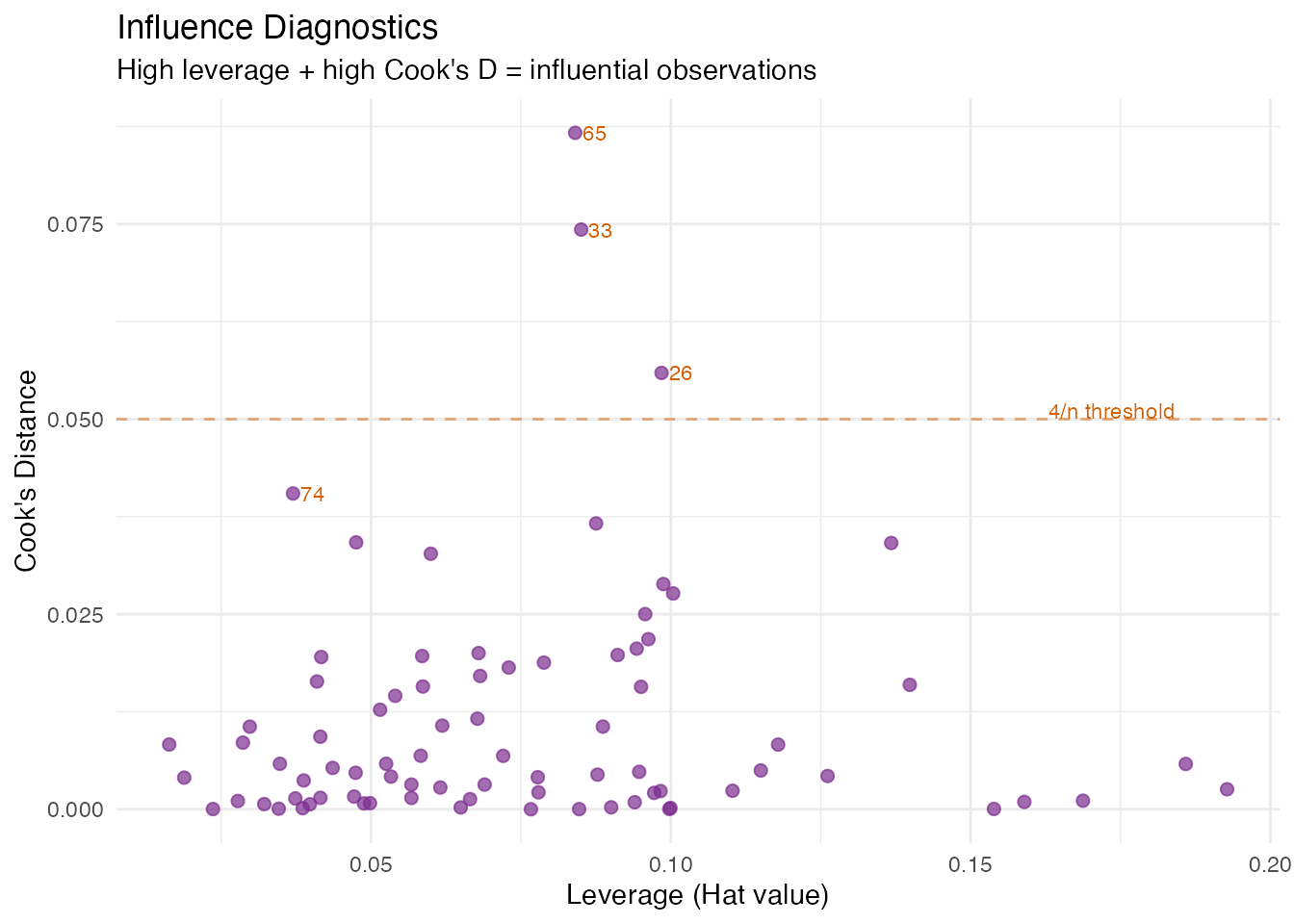

Leverage Distribution

Observations above the dashed threshold have FPC scores far from the centroid. In an industrial setting, these might be sensors operating under unusual conditions.

ggplot(df_inf, aes(x = .data$Observation, y = .data$Leverage)) +
  geom_segment(aes(xend = .data$Observation, yend = 0), color = "gray70") +
  geom_point(color = "#4A90D9", size = 2) +
  geom_hline(yintercept = 2 * (model$ncomp + 1) / n, linetype = "dashed",
             color = "#D55E00") +
  labs(title = "Leverage per Observation",
       subtitle = paste("Threshold: 2(K+1)/n =",
                        round(2 * (model$ncomp + 1) / n, 3)),
       x = "Observation", y = "Leverage")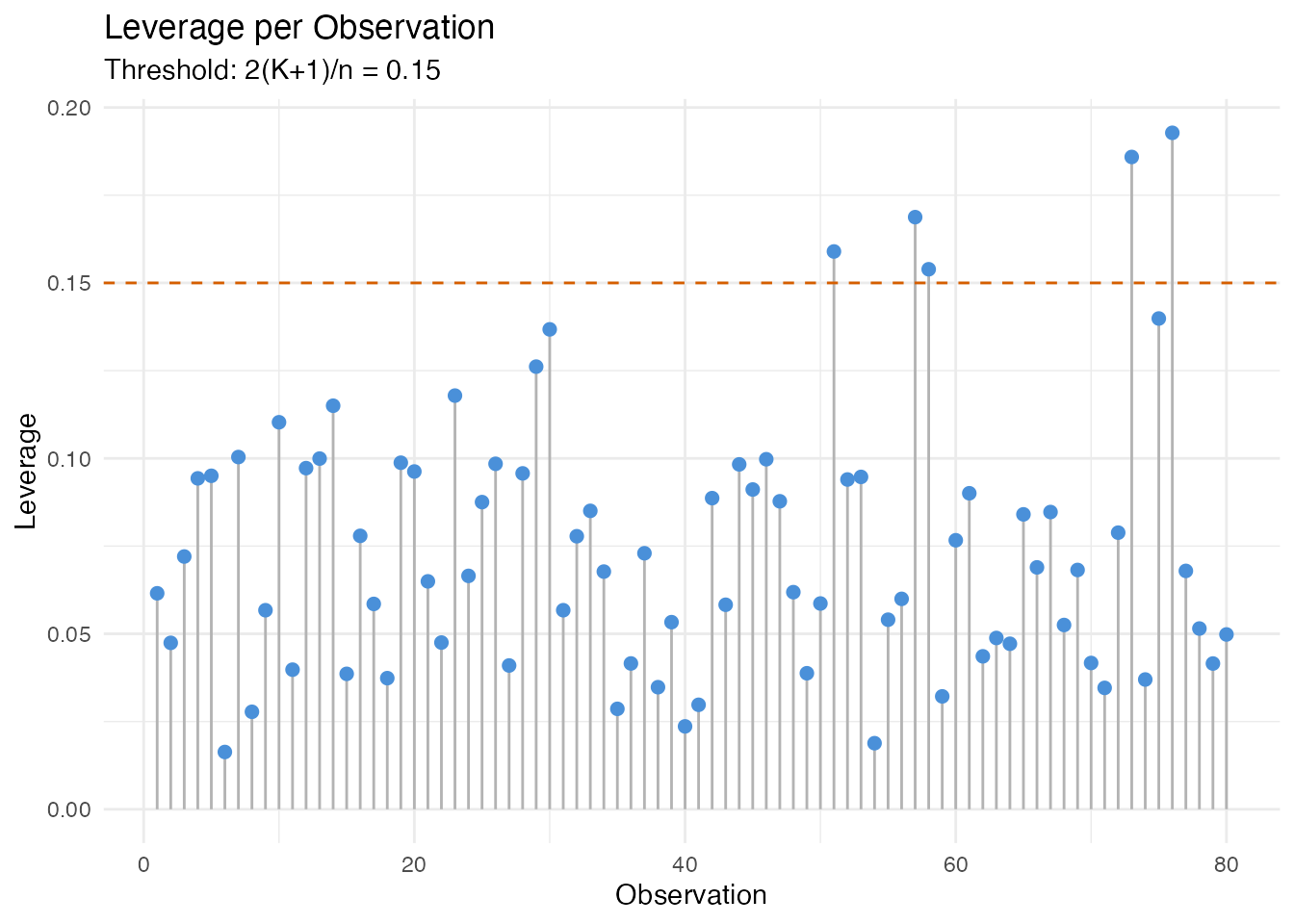

DFBETAS and DFFITS

In plain English: DFBETAS asks, for each observation and each regression coefficient: “how much would this coefficient change if I removed this observation?” DFFITS is similar but for the fitted value itself: “how much would observation $i$ ’s prediction change if I refitted without it?”

Large DFBETAS values for a specific component indicate that the observation is driving that component’s regression coefficient. This helps pinpoint which aspect of the model an influential point affects, not just that it matters.

Mathematically:

$\text{DFBETAS}_{ij} = \frac{\hat{b}_j - \hat{b}_j^{(-i)}}{\hat{\sigma}^{(-i)}\sqrt{(\boldsymbol{\Xi}^\top\boldsymbol{\Xi})^{-1}_{jj}}},$

$\text{DFFITS}_i = \frac{\hat{y}_i - \hat{y}_i^{(-i)}}{\hat{\sigma}^{(-i)}\sqrt{h_{ii}}}.$

The standard cutoff for DFBETAS is $2/\sqrt{n}$ ; for DFFITS it is $2\sqrt{(K+1)/n}$ .

dfb <- fregre.dfbetas(model, data = fdataobj)

cat("DFBETAS cutoff (2/sqrt(n)):", round(dfb$dfbetas_cutoff, 3), "\n")
#> DFBETAS cutoff (2/sqrt(n)): 0.224
cat("DFFITS cutoff:", round(dfb$dffits_cutoff, 3), "\n")
#> DFFITS cutoff: 0.548

df_dffits <- data.frame(
  Observation = seq_len(n),
  DFFITS = dfb$dffits
)

ggplot(df_dffits, aes(x = .data$Observation, y = abs(.data$DFFITS))) +
  geom_segment(aes(xend = .data$Observation, yend = 0), color = "gray70") +
  geom_point(color = "#7B2D8E", size = 2) +
  geom_hline(yintercept = dfb$dffits_cutoff, linetype = "dashed",
             color = "#D55E00") +
  labs(title = "DFFITS: Case Influence on Fitted Values",
       subtitle = paste("Cutoff:", round(dfb$dffits_cutoff, 3)),
       x = "Observation", y = "|DFFITS|")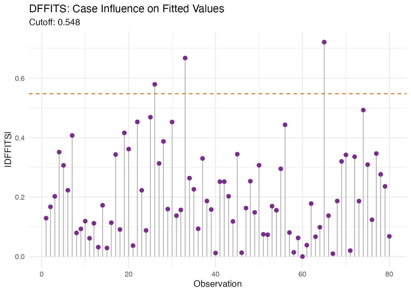

ncomp_show <- min(3, ncol(dfb$dfbetas))
df_dfb <- do.call(rbind, lapply(seq_len(ncomp_show), function(k) {
  data.frame(Observation = seq_len(n),
             DFBETAS = dfb$dfbetas[, k],
             Component = paste0("PC", k))
}))

ggplot(df_dfb, aes(x = .data$Observation, y = .data$DFBETAS)) +
  geom_point(color = "#4A90D9", size = 1.5, alpha = 0.6) +
  geom_hline(yintercept = c(-dfb$dfbetas_cutoff, dfb$dfbetas_cutoff),
             linetype = "dashed", color = "#D55E00") +
  facet_wrap(~ Component) +
  labs(title = "DFBETAS per FPC Component",
       subtitle = "Per-coefficient case influence — points beyond cutoff shift that coefficient",
       x = "Observation", y = "DFBETAS")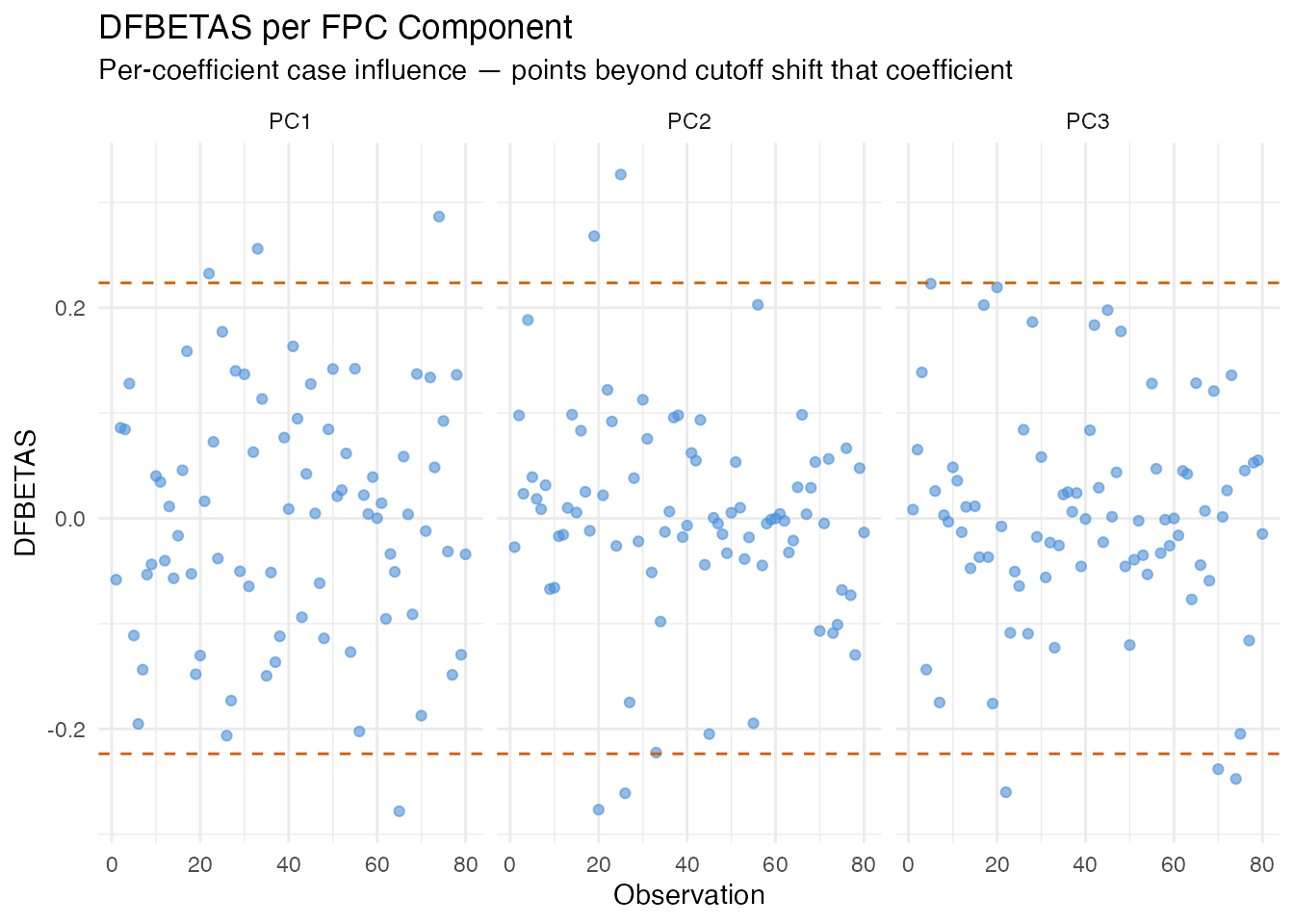

Variance Inflation Factor

In plain English: VIF checks whether the FPC scores are collinear with each other (or with scalar covariates). If two predictors carry the same information, the regression coefficients become unstable. Since FPC scores are orthogonal by construction, VIF should be near 1 for a pure FPCA model. VIF > 5 indicates a problem — typically when scalar covariates correlate with FPC scores or when the score matrix is numerically ill-conditioned.

Mathematically: The VIF for score $k$ is

$\text{VIF}_k = \frac{1}{1 - R_k^2},$

where $R_k^2$ is the $R^2$ from regressing $\xi_k$ on all other predictors. VIF = 1 means no collinearity; VIF = 10 means 90% of the variance of $\xi_k$ is explained by other predictors.

Supported models: fregre.lm + functional.logistic.

vif_scores <- fregre.vif(model, data = fdataobj)

df_vif <- data.frame(
  Component = paste0("PC", seq_along(vif_scores$vif)),
  VIF = vif_scores$vif
)

ggplot(df_vif, aes(x = .data$Component, y = .data$VIF)) +
  geom_col(fill = "#7B2D8E", alpha = 0.7) +
  geom_hline(yintercept = 5, linetype = "dashed", color = "#D55E00") +
  annotate("text", x = length(vif_scores$vif), y = 5.3,
           label = "VIF = 5 threshold", color = "#D55E00", hjust = 1, size = 3) +
  labs(title = "Variance Inflation Factor",
       subtitle = paste("Mean VIF:", round(vif_scores$mean_vif, 2),
                        "— values near 1 confirm orthogonal FPC scores"),
       x = "Component", y = "VIF")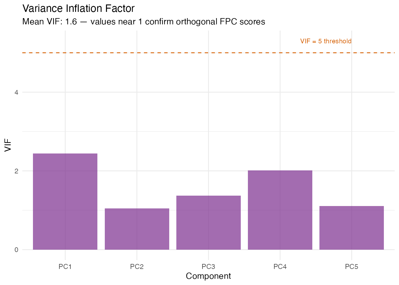

Residual Diagnostics

Standard regression diagnostics check the model assumptions visually. These plots use only the fregre.lm model’s residuals and fitted values.

Residuals vs Fitted

In plain English: If the model is well-specified, residuals should scatter randomly around zero with constant spread. Patterns (curves, funnels) indicate model misspecification: a curve means a nonlinear effect is missing; a funnel means heteroscedasticity (variance changes with the fitted value). Point size encodes leverage, so large distant points are the most concerning.

df_resid <- data.frame(
  Fitted = model$fitted.values,
  Residual = model$residuals,
  Leverage = influence$leverage
)

ggplot(df_resid, aes(x = .data$Fitted, y = .data$Residual)) +
  geom_point(aes(size = .data$Leverage), color = "#4A90D9", alpha = 0.6) +
  geom_hline(yintercept = 0, linetype = "dashed") +
  geom_smooth(method = "loess", se = FALSE, color = "#D55E00", linewidth = 0.8) +
  scale_size_continuous(range = c(1, 5)) +
  labs(title = "Residuals vs Fitted Values",
       subtitle = "Point size = leverage; orange line = loess smoother (should be flat at zero)",
       x = "Fitted Values", y = "Residuals")
#> `geom_smooth()` using formula = 'y ~ x'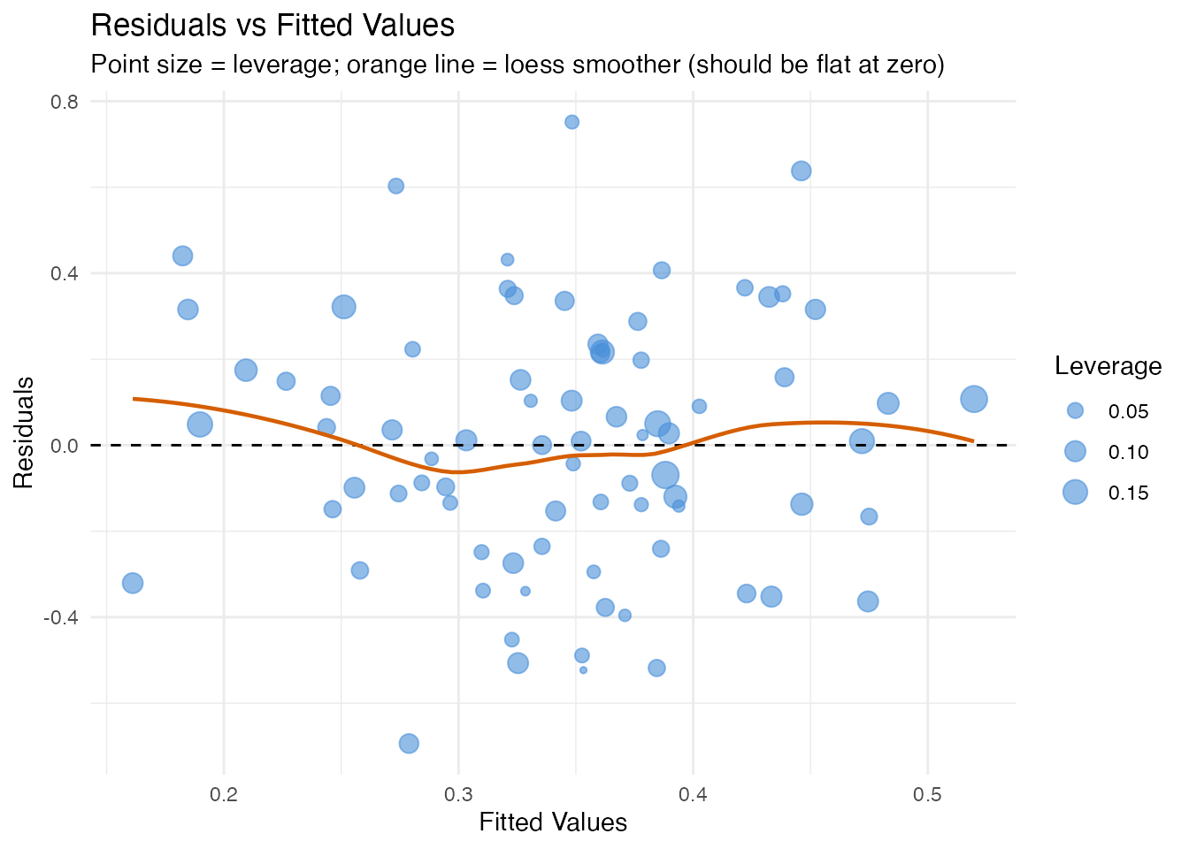

Normal Q-Q Plot

In plain English: If the errors are normally distributed, the points follow the diagonal line. Deviations at the tails indicate heavy tails (outliers) or skewness. Normality is assumed by prediction intervals (see the uncertainty quantification article) but not by conformal prediction.

df_qq <- data.frame(Residual = model$residuals)

ggplot(df_qq, aes(sample = .data$Residual)) +
  stat_qq(color = "#4A90D9", size = 2, alpha = 0.7) +
  stat_qq_line(color = "#D55E00") +
  labs(title = "Normal Q-Q Plot of Residuals",
       subtitle = "Points on the line = Gaussian residuals; tails off = heavy tails / skewness",
       x = "Theoretical Quantiles", y = "Sample Quantiles")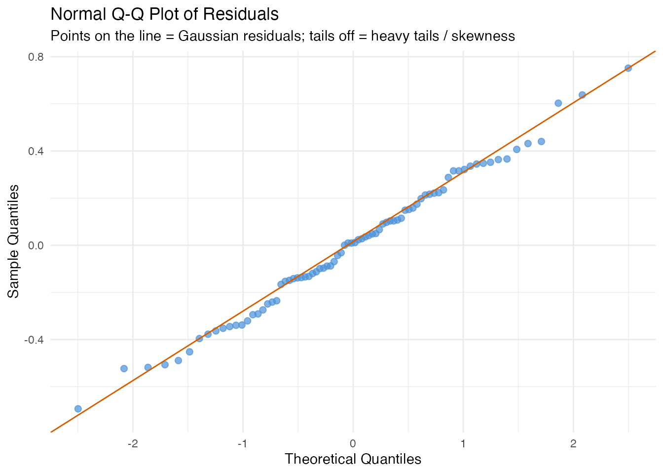

Scale-Location Plot

In plain English: This plot checks for heteroscedasticity from a different angle. The y-axis shows $\sqrt{|e_i|}$ against fitted values. If the spread is constant, the smoother should be roughly flat.

df_sl <- data.frame(
  Fitted = model$fitted.values,
  SqrtAbsResid = sqrt(abs(model$residuals))
)

ggplot(df_sl, aes(x = .data$Fitted, y = .data$SqrtAbsResid)) +
  geom_point(color = "#2E8B57", size = 2, alpha = 0.6) +
  geom_smooth(method = "loess", se = FALSE, color = "#D55E00", linewidth = 0.8) +
  labs(title = "Scale-Location Plot",
       subtitle = "Flat smoother = constant variance (homoscedasticity)",
       x = "Fitted Values", y = expression(sqrt("|Residual|")))
#> `geom_smooth()` using formula = 'y ~ x'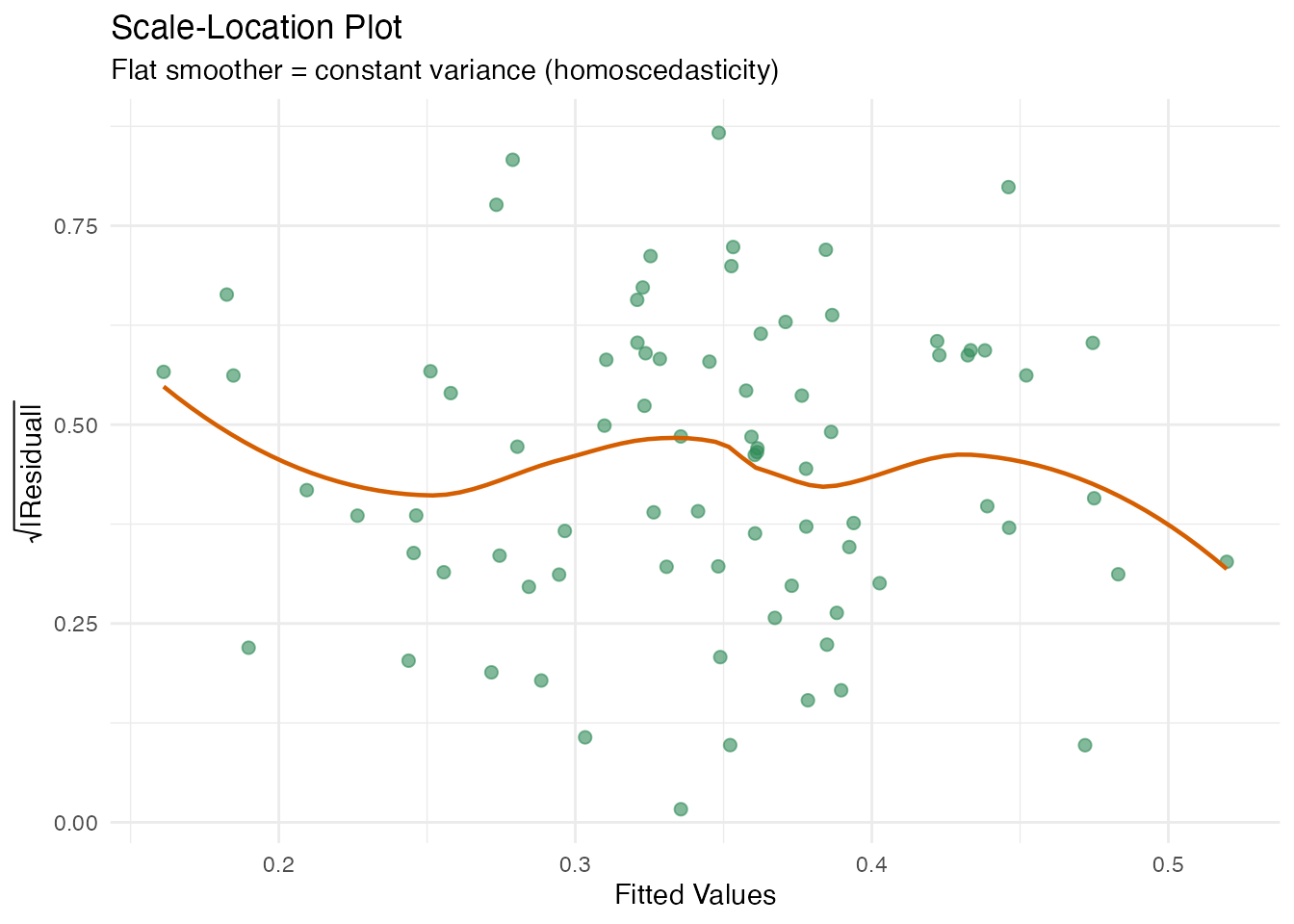

Importance and Robustness

These methods assess which FPC scores matter and how stable the model is.

Supported models: fregre.lm + functional.logistic (except stability, which is model-free).

Permutation Importance

In plain English: For each FPC score, we randomly shuffle its values (breaking the relationship with $y$ ) and measure how much the prediction error increases. A large increase means the model relies heavily on that score. This is a model-agnostic importance measure (works for any model that predicts from FPC scores).

Mathematically: The importance of score $k$ is

$\text{Imp}_k = \frac{1}{P}\sum_{p=1}^{P}\left[\text{MSE}(\hat{y};\,\tilde{\xi}_k^{(p)}) - \text{MSE}(\hat{y})\right],$

where $\tilde{\xi}_k^{(p)}$ is the $p$ -th random permutation of score $k$ and $P$ is the number of permutation replicates. The importance is always non-negative for a useful predictor.

imp <- fregre.importance(model, data = fdataobj, y = y, n.perm = 50, seed = 42)

df_imp <- data.frame(
  Component = paste0("PC", seq_along(imp$importance)),
  Importance = imp$importance
)

ggplot(df_imp, aes(x = reorder(.data$Component, -.data$Importance),
                   y = .data$Importance)) +
  geom_col(fill = "#4A90D9", alpha = 0.7) +
  labs(title = "Permutation Importance",
       subtitle = paste("Baseline MSE:", round(imp$baseline_metric, 4),
                        "— bars show MSE increase when shuffling each score"),
       x = "Component", y = "Importance (MSE increase)")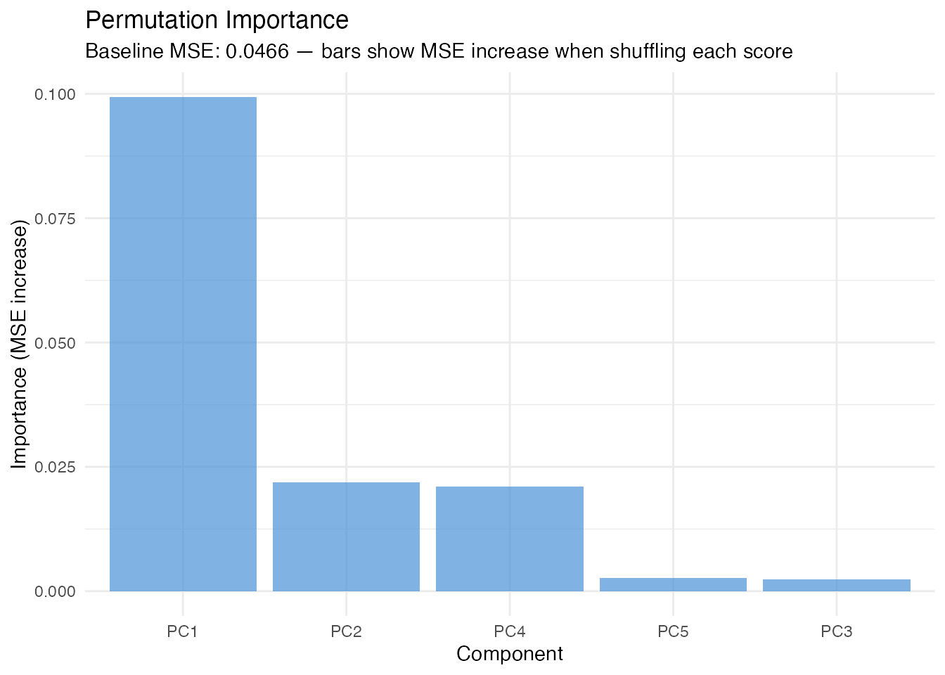

Conditional Permutation Importance

In plain English: Standard permutation importance can overstate a score’s importance when predictors are correlated, because shuffling one score implicitly breaks its correlation with other scores. Conditional permutation fixes this by shuffling within bins of the other predictors, preserving the correlation structure. The difference between unconditional and conditional importance reveals how much of a score’s apparent importance comes from correlation rather than direct prediction.

Mathematically: Instead of permuting $\xi_k$ freely, we partition the other scores $\boldsymbol{\xi}_{-k}$ into $B$ bins and permute $\xi_k$ only within observations that share the same bin. This keeps the conditional distribution $\xi_k \mid \boldsymbol{\xi}_{-k}$ approximately intact.

Since FPC scores are orthogonal by construction, conditional and unconditional importance should agree closely here. When scalar covariates are included, they may diverge.

cimp <- fregre.conditional.importance(model, data = fdataobj, y = y,
                                      n.bins = 5, n.perm = 50, seed = 42)

df_cimp <- data.frame(
  Component = paste0("PC", seq_along(cimp$importance)),
  Conditional = cimp$importance,
  Unconditional = cimp$unconditional_importance
)
df_cimp_long <- rbind(
  data.frame(Component = df_cimp$Component, Value = df_cimp$Conditional,
             Type = "Conditional"),
  data.frame(Component = df_cimp$Component, Value = df_cimp$Unconditional,
             Type = "Unconditional")
)

ggplot(df_cimp_long, aes(x = .data$Component, y = .data$Value,
                         fill = .data$Type)) +
  geom_col(position = "dodge", alpha = 0.7) +
  scale_fill_manual(values = c("Conditional" = "#4A90D9",
                                "Unconditional" = "#D55E00")) +
  labs(title = "Conditional vs Unconditional Permutation Importance",
       subtitle = "Similar values confirm FPC scores are orthogonal (no spurious importance)",
       x = "Component", y = "Importance") +
  theme(legend.position = "bottom")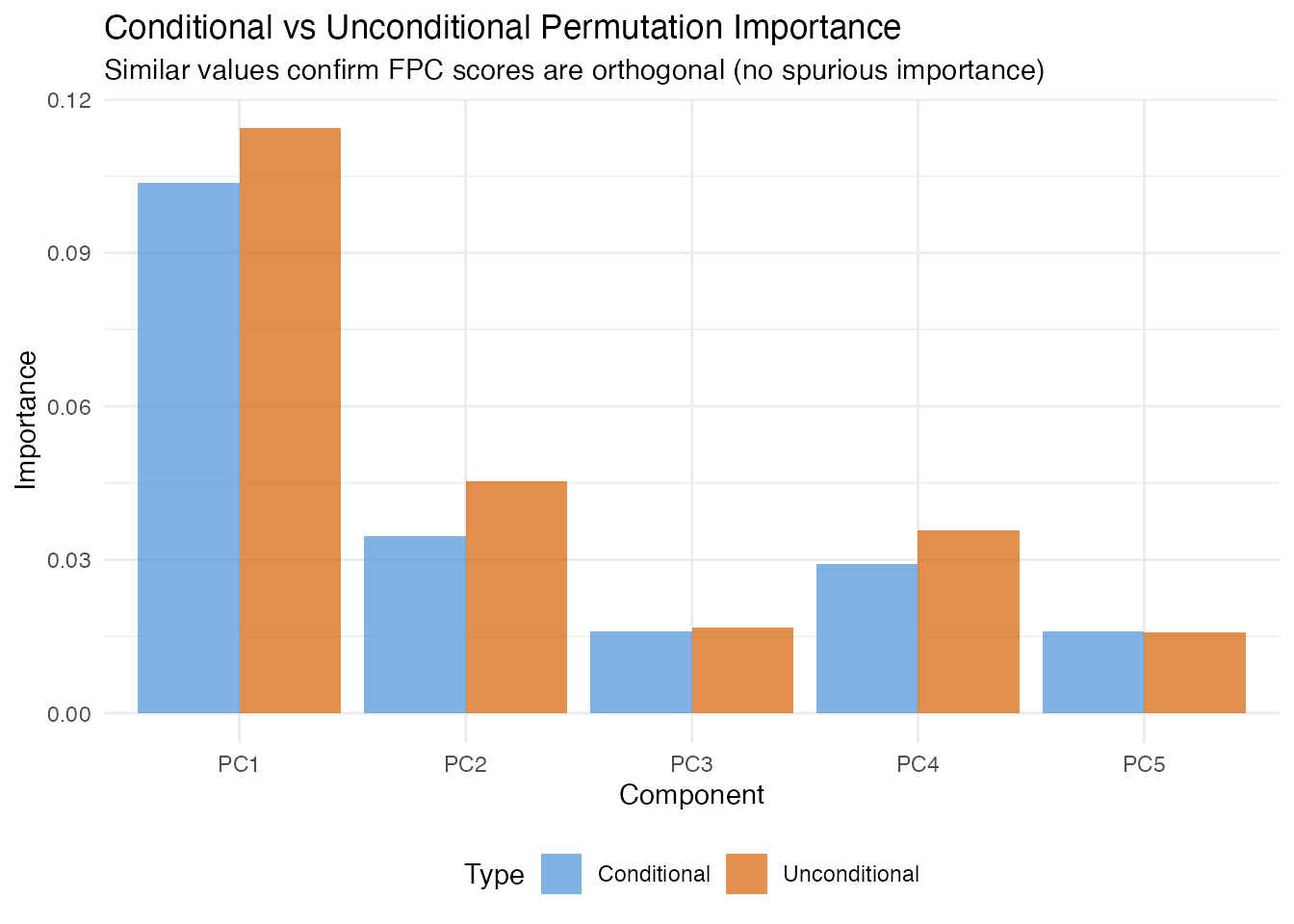

Regression Depth

In plain English: Regression depth measures how “central” the estimated coefficient vector is among bootstrap resamples. A high depth means the estimate sits near the middle of the bootstrap cloud — it is robust. A low depth means it is near the boundary, suggesting that a small data perturbation could substantially change the coefficients. This is particularly useful for detecting sensitivity to outliers.

Mathematically: Given $B$ bootstrap replicates $\hat{\boldsymbol{b}}^{*(1)},\ldots,\hat{\boldsymbol{b}}^{*(B)}$ , the regression depth of $\hat{\boldsymbol{b}}$ is the minimum fraction of bootstrap replicates that lie on one side of any hyperplane through $\hat{\boldsymbol{b}}$ . Depth ranges from 0 (boundary) to 0.5 (deepest possible).

The per-component score depths reveal which specific coefficients are most and least stable.

rdepth <- fregre.depth(model, data = fdataobj, y = y, n.boot = 50, seed = 42)

cat("Beta depth:", round(rdepth$beta_depth, 4), "\n")
#> Beta depth: 0.328
cat("Mean score depth:", round(rdepth$mean_score_depth, 4), "\n")
#> Mean score depth: 0.25
cat("Bootstrap replicates:", rdepth$n_boot_success, "\n")
#> Bootstrap replicates: 50

df_sdepth <- data.frame(
  Component = paste0("PC", seq_along(rdepth$score_depths)),
  Depth = rdepth$score_depths
)

ggplot(df_sdepth, aes(x = .data$Component, y = .data$Depth)) +
  geom_col(fill = "#2E8B57", alpha = 0.7) +
  labs(title = "Score-Level Regression Depth",
       subtitle = "Higher = more robust; low depth = sensitive to data perturbations",
       x = "Component", y = "Depth")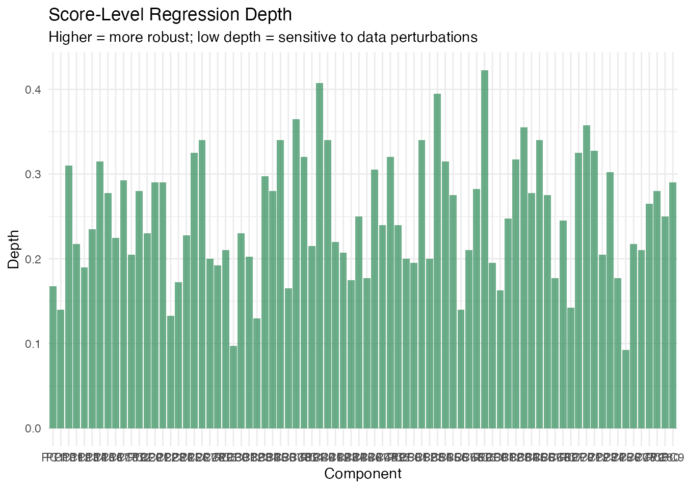

Explanation Stability

In plain English: Stability analysis asks: “if I collected a slightly different sample, how much would $\beta(t)$ change?” It bootstraps the entire model-fitting process (FPCA + regression) and computes the coefficient of variation (CV) of $\hat{\beta}(t)$ at each domain point. Low CV means the coefficient is stable; high CV means it fluctuates across samples and should be interpreted cautiously.

Mathematically: For $B$ bootstrap resamples, the pointwise CV is

$\text{CV}(t) = \frac{\hat{\sigma}_{\text{boot}}(\hat{\beta}(t))}{|\overline{\hat{\beta}}(t)| + \epsilon},$

where $\hat{\sigma}_{\text{boot}}$ is the bootstrap standard deviation and $\epsilon$ is a small constant to avoid division by zero near $\beta(t) = 0$ .

Model-free: This function takes data, y, ncomp rather than a fitted model, because it refits the model from scratch on each bootstrap sample.

stab <- fregre.stability(data = fdataobj, y = y, ncomp = 5,
                         n.boot = 50, seed = 42)

cat("Mean beta(t) CV:", round(mean(stab$beta_t_cv), 4), "\n")
#> Mean beta(t) CV: 24.539
cat("Coefficient std devs:", round(stab$coefficient_std, 4), "\n")
#> Coefficient std devs: 0.2045 2.1157 2.0746 1.9139 2.5343
cat("Bootstrap successes:", stab$n_boot_success, "\n")
#> Bootstrap successes: 50

df_stab <- data.frame(t = t_grid, cv = stab$beta_t_cv)

ggplot(df_stab, aes(x = .data$t, y = .data$cv)) +
  geom_line(color = "#C0392B", linewidth = 1) +
  geom_ribbon(aes(ymin = 0, ymax = .data$cv), fill = "#C0392B", alpha = 0.1) +
  labs(title = "Coefficient of Variation for beta(t)",
       subtitle = "Lower = more stable; peaks indicate unreliable regions",
       x = "t", y = "CV")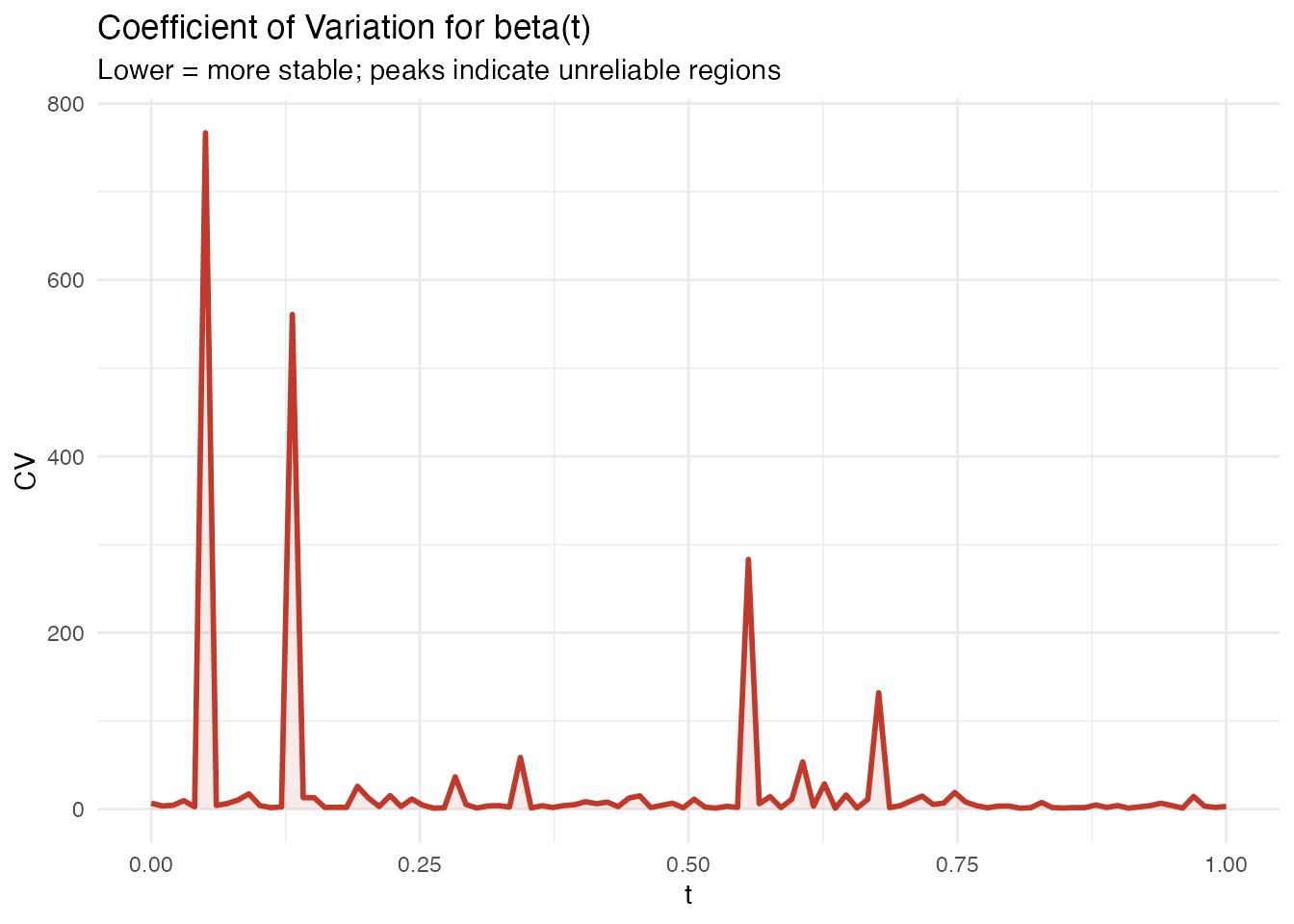

Summary

Diagnostic	Question	Model	Key threshold
Leverage	How unusual is this curve’s shape?	lm	$h_{ii} > 2(K+1)/n$
Cook’s D	How much does removing this observation change the fit?	lm	$D_i > 4/n$
DFBETAS	Which coefficient does this observation affect?	lm	$> 2/\sqrt{n}$
DFFITS	How much does the fitted value change?	lm	$> 2\sqrt{(K+1)/n}$
VIF	Are the FPC scores collinear?	lm, logistic	VIF > 5
Permutation importance	Which scores drive predictions?	lm, logistic	Relative ranking
Conditional importance	Same, corrected for correlations	lm, logistic	Relative ranking
Regression depth	Is the coefficient estimate robust?	lm, logistic	Near 0.5 = robust
Stability CV	Does $\beta(t)$ change across samples?	model-free	Low CV = stable

References

Belsley, D.A., Kuh, E. and Welsch, R.E. (1980). Regression Diagnostics. Wiley.
Breiman, L. (2001). Random forests. Machine Learning, 45(1), 5–32.
Cook, R.D. (1977). Detection of influential observations in linear regression. Technometrics, 19(1), 15–18.
Kutner, M.H., Nachtsheim, C.J., Neter, J. and Li, W. (2004). Applied Linear Statistical Models. 5th ed. McGraw-Hill/Irwin.
Ramsay, J.O. and Silverman, B.W. (2005). Functional Data Analysis. 2nd ed. Springer.
Rousseeuw, P.J. and Hubert, M. (1999). Regression depth. Journal of the American Statistical Association, 94(446), 388–402.
Strobl, C., Boulesteix, A.-L., Kneib, T., Augustin, T. and Zeileis, A. (2008). Conditional variable importance for random forests. BMC Bioinformatics, 9, 307.