Advanced Elastic Alignment

Introduction

This article covers the advanced alignment methods introduced in fdars-core 0.10.0. These extend the foundational elastic alignment framework (see Elastic Curve Alignment) with robust estimation, uncertainty quantification, specialized geometries, and diagnostic tools.

All methods operate on the elastic manifold defined by the Square-Root Slope Function (SRSF) representation $q(t) = \text{sign}(\dot{f}(t)) \sqrt{|\dot{f}(t)|}$ , which converts the Fisher-Rao metric to the $L^2$ metric on the Hilbert sphere (Srivastava et al., 2011).

library(fdars)
#> 
#> Attaching package: 'fdars'
#> The following objects are masked from 'package:stats':
#> 
#>     cov, decompose, deriv, median, sd, var
#> The following object is masked from 'package:base':
#> 
#>     norm
library(ggplot2)
library(patchwork)
theme_set(theme_minimal())
set.seed(42)

# Simulated curves with amplitude and phase variability
n <- 30
t_grid <- seq(0, 1, length.out = 200)
fd_list <- lapply(seq_len(n), function(i) {
  amp <- rnorm(1, 3, 0.5)
  shift <- rnorm(1, 0.5, 0.08)
  noise <- cumsum(rnorm(200, 0, 0.02))
  amp * dnorm(t_grid, mean = shift, sd = 0.12) + noise
})
fd <- fdata(do.call(rbind, fd_list), argvals = t_grid)

1. Robust Karcher Mean and Median

Motivation

The standard Karcher mean minimizes the sum of squared elastic distances and is sensitive to outlier curves. For contaminated data, two alternatives exist:

Karcher median: minimizes the sum of (unsquared) distances via the Weiszfeld algorithm on the elastic manifold – the functional analog of the geometric median.
Trimmed Karcher mean: removes the most distant curves before computing the mean.

Mathematical Background

The Karcher median on a Riemannian manifold $M$ is defined as:

$\tilde{\mu} = \arg\min_{\mu \in M} \sum_{i=1}^{n} d(\mu, f_i)$

This is solved iteratively using the Weiszfeld algorithm adapted to manifolds (Fletcher et al., 2009): at each step, compute the weighted Frechet mean where weights are inversely proportional to distances from the current estimate.

The trimmed Karcher mean removes the $k$ most distant curves (in elastic distance) before computing the standard Karcher mean, following the approach of Cuesta-Albertos & Fraiman (2007) extended to the elastic manifold.

# Standard Karcher mean (reference)
km <- karcher.mean(fd, max.iter = 15)

# Karcher median (robust to outliers)
kmed <- karcher.median(fd, max.iter = 15)

# Trimmed Karcher mean (remove 10% most distant curves)
km_trimmed <- robust.karcher.mean(fd, trim = 0.1, max.iter = 15)

# Compare the three estimates
km_vals <- as.numeric(km$mean$data[1, ])
kmed_vals <- as.numeric(kmed$mean$data[1, ])
ktrim_vals <- as.numeric(km_trimmed$mean$data[1, ])
# Ensure all same length (use km argvals as reference)
km_t <- as.numeric(km$mean$argvals)
df_means <- data.frame(
  t = rep(km_t, 3),
  value = c(km_vals, kmed_vals[seq_along(km_vals)],
            ktrim_vals[seq_along(km_vals)]),
  method = rep(c("Karcher Mean", "Karcher Median", "Trimmed Mean (10%)"),
               each = length(km_t))
)
ggplot(df_means, aes(x = .data$t, y = .data$value, color = .data$method)) +
  geom_line(linewidth = 0.8) +
  labs(title = "Robust vs Standard Karcher Mean",
       x = "t", y = "f(t)", color = NULL) +
  theme(legend.position = "bottom")
#> Warning: Removed 200 rows containing missing values or values outside the scale range
#> (`geom_line()`).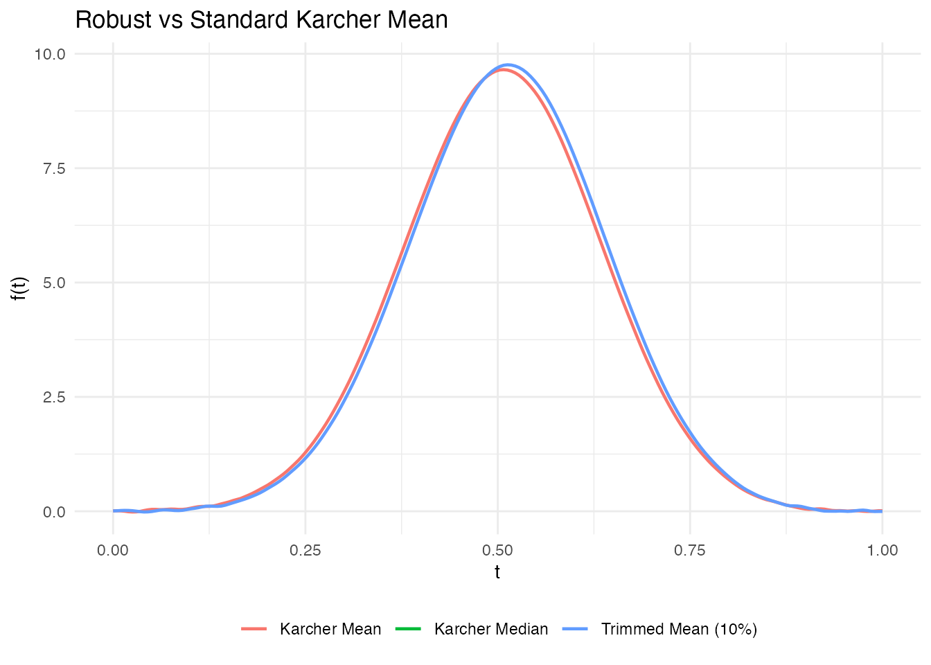

References:

Fletcher, P. T., Venkatasubramanian, S., & Joshi, S. (2009). The geometric median on Riemannian manifolds with application to robust atlas estimation. NeuroImage, 45(1), S143–S152. DOI: 10.1016/j.neuroimage.2008.10.052
Cuesta-Albertos, J. A. & Fraiman, R. (2007). Impartial trimmed k-means for functional data. Computational Statistics & Data Analysis, 51(10), 4864–4877.

2. Elastic Depth

Motivation

Functional depth measures how “central” a curve is in a sample. Standard depth (e.g., MBD) ignores phase variability – two curves may have similar depth despite one being time-warped. Elastic depth decomposes the depth into amplitude and phase components using elastic distances.

Method

For each curve $f_i$ , the elastic depth is computed as:

$D_{\text{elastic}}(f_i) = \frac{1}{1 + \bar{d}_{\text{elastic}}(f_i)}$

where $\bar{d}_{\text{elastic}}(f_i)$ is the average elastic distance from $f_i$ to all other curves. The decomposition into amplitude and phase depths uses the aligned vs unaligned distances:

Amplitude depth: based on $L^2$ distances after alignment
Phase depth: based on the warping function complexity

# Elastic depth with amplitude/phase decomposition
ed <- elastic.depth(fd)

cat("Amplitude depth range:", round(range(ed$amplitude_depth), 3), "\n")
#> Amplitude depth range: 0.48 0.556
cat("Phase depth range:    ", round(range(ed$phase_depth), 3), "\n")
#> Phase depth range:     0.734 0.772
cat("Combined depth range: ", round(range(ed$combined_depth), 3), "\n")
#> Combined depth range:  0.6 0.652
cat("Deepest curve (most central):", which.max(ed$combined_depth), "\n")
#> Deepest curve (most central): 11

References:

Lopez-Pintado, S. & Romo, J. (2009). On the concept of depth for functional data. Journal of the American Statistical Association, 104(486), 718–734. DOI: 10.1198/jasa.2009.0108
Srivastava, A. & Klassen, E. P. (2016). Functional and Shape Data Analysis. Springer. Chapter 9: Statistical Summaries.

3. SRVF Outlier Detection

Motivation

Outlier detection in the elastic framework accounts for both amplitude and phase anomalies. A curve can be an outlier because it has an unusual shape (amplitude outlier), an unusual timing (phase outlier), or both.

Method

Elastic outlier detection computes the distance from each curve to a reference (mean or median) and applies Tukey fence thresholding:

$\text{outlier if } d_{\text{elastic}}(f_i, \mu) > Q_3 + k \cdot \text{IQR}$

where $k$ is typically 1.5. The amplitude/phase decomposition classifies outliers into types.

# Outlier detection with amplitude/phase decomposition
outliers <- elastic.outlier.detection(fd)

cat("Outlier indices:", if (length(outliers$outlier_indices) > 0)
  paste(outliers$outlier_indices, collapse = ", ") else "none", "\n")
#> Outlier indices: none
cat("Threshold:", round(outliers$threshold, 4), "\n")
#> Threshold: 1.0662
cat("Distance range:", round(range(outliers$distances), 4), "\n")
#> Distance range: 0.4751 0.8892

References:

Xie, W., Kurtek, S., Bharath, K., & Sun, Y. (2017). A geometric approach to visualization of variability in functional data. Journal of the American Statistical Association, 112(519), 979–993. DOI: 10.1080/01621459.2016.1256813
Dai, W. & Genton, M. G. (2018). Functional boxplots. Journal of Computational and Graphical Statistics, 20(2), 316–334.

4. Shape Confidence Intervals

Motivation

After computing the Karcher mean, how certain are we about its shape? Shape confidence intervals provide bootstrap confidence bands for the elastic mean, quantifying estimation uncertainty.

Method

Resample $B$ bootstrap samples from the original curves
For each sample, compute the Karcher mean
Align all bootstrap means to the original mean
Compute pointwise percentile bands (e.g., 2.5% and 97.5%)

The alignment step is crucial: without it, phase variability between bootstrap means inflates the bands artificially.

# Bootstrap confidence bands for the Karcher mean
ci <- shape.confidence.interval(fd, n.bootstrap = 50, max.iter = 10)

df_ci <- data.frame(
  t = rep(t_grid, 3),
  value = c(ci$lower_band, as.numeric(ci$mean$data[1, ]), ci$upper_band),
  type = rep(c("Lower 95%", "Mean", "Upper 95%"), each = length(t_grid))
)

ggplot(df_ci, aes(x = .data$t, y = .data$value, linetype = .data$type)) +
  geom_line(color = "#4A90D9", linewidth = 0.8) +
  scale_linetype_manual(values = c("Lower 95%" = "dashed",
                                    "Mean" = "solid",
                                    "Upper 95%" = "dashed")) +
  labs(title = "Shape Confidence Interval for Karcher Mean",
       x = "t", y = "f(t)", linetype = NULL) +
  theme(legend.position = "bottom")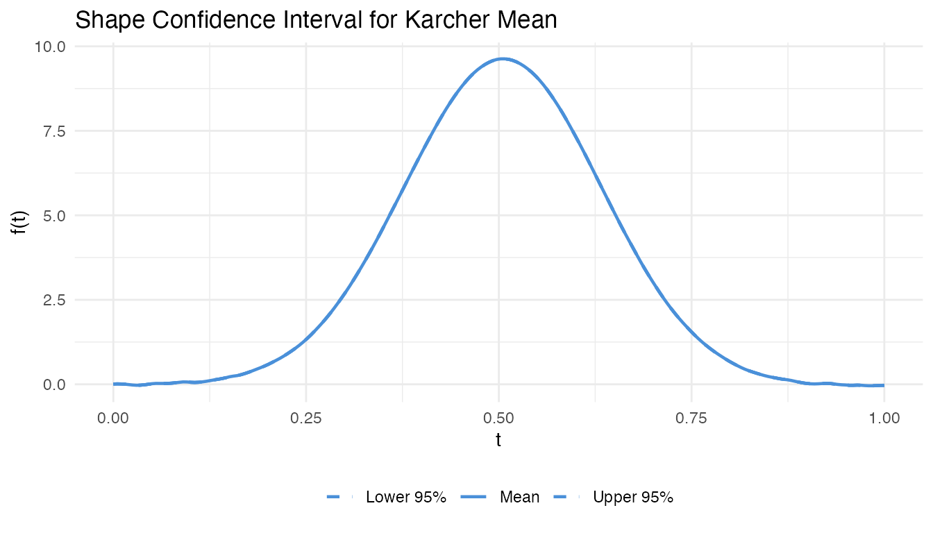

References:

Kurtek, S. & Marron, J. S. (2017). Elastic shape analysis of boundaries of planar objects. Annals of Applied Statistics, 11(3), 1490–1521. DOI: 10.1214/17-AOAS1059
Srivastava, A. & Klassen, E. P. (2016). Functional and Shape Data Analysis. Springer. Chapter 8: Statistical Analysis of Shapes.

5. Bayesian Alignment

Motivation

Standard dynamic programming alignment yields a point estimate of the warping function. Bayesian alignment provides a posterior distribution over warping functions, enabling uncertainty quantification: credible bands on aligned curves, posterior predictive distributions, and model comparison.

Method

The method uses the preconditioned Crank-Nicolson (pCN) MCMC sampler on the Hilbert sphere (Cotter et al., 2013), adapted for functional alignment by Cheng et al. (2016). The prior over warping functions is a Dirichlet process or Gaussian process on the sphere of SRSFs; the likelihood measures the $L^2$ fit between the SRSFs after warping.

The pCN proposal

$\gamma^* = \sqrt{1 - \beta^2} \, \gamma^{(k)} + \beta \, \xi, \quad \xi \sim \Pi_0$

ensures dimension-independent acceptance rates, making the algorithm scalable to fine time grids.

# Bayesian alignment of two curves
ba <- bayesian.align.pair(fd$data[1, ], fd$data[2, ],
                           argvals = t_grid,
                           n.samples = 500, burn.in = 100)

cat("Acceptance rate:", round(ba$acceptance_rate, 3), "\n")
#> Acceptance rate: 0.802

# Plot original vs Bayesian-aligned
df_ba <- data.frame(
  t = rep(t_grid, 3),
  value = c(fd$data[1, ], fd$data[2, ], ba$f_aligned_mean),
  curve = rep(c("f1 (reference)", "f2 (original)", "f2 (Bayesian aligned)"),
              each = length(t_grid))
)
ggplot(df_ba, aes(x = .data$t, y = .data$value, color = .data$curve)) +
  geom_line(linewidth = 0.8) +
  labs(title = "Bayesian Pairwise Alignment",
       subtitle = sprintf("Acceptance rate: %.1f%%", 100 * ba$acceptance_rate),
       x = "t", y = "f(t)", color = NULL) +
  theme(legend.position = "bottom")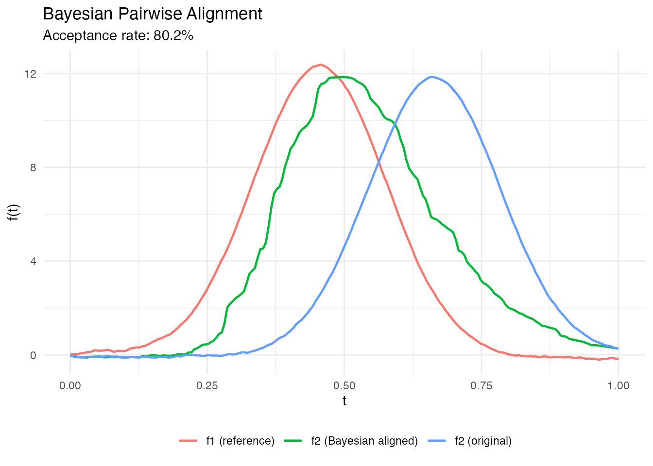

References:

Cheng, W., Dryden, I. L., & Huang, X. (2016). Bayesian registration of functions and curves. Bayesian Analysis, 11(2), 447–481. DOI: 10.1214/15-BA957
Cotter, S. L., Roberts, G. O., Stuart, A. M., & White, D. (2013). MCMC methods for functions: modifying old algorithms to make them faster. Statistical Science, 28(3), 424–446. DOI: 10.1214/13-STS421
Lu, Y., Herbei, R., & Kurtek, S. (2017). Bayesian registration of functions with a Gaussian process prior. Journal of Computational and Graphical Statistics, 26(4), 894–904.

6. Multi-Resolution Alignment

Motivation

Dynamic programming alignment has $O(T^2)$ complexity, making it slow for long curves ( $T > 1000$ ). Multi-resolution alignment performs a coarse alignment on a subsampled grid, then refines on the original resolution – achieving near-optimal alignment in $O(T \log T)$ time.

Method

Coarse stage: Subsample the curve to $T/k$ points and run DP alignment to get an approximate warping path
Fine stage: Use the coarse warp as initialization for gradient refinement (e.g., L-BFGS) on the full-resolution grid

This is related to the FastDTW approach (Salvador & Chan, 2007) but adapted to the elastic (SRSF) framework.

# Multi-resolution alignment (faster for long curves)
mr <- elastic.align.pair.multires(fd$data[1, ], fd$data[2, ],
                                   argvals = t_grid,
                                   coarsen.factor = 4)

cat("Multi-res distance:", round(mr$distance, 4), "\n")
#> Multi-res distance: 1.0429

# Compare with standard DP alignment
std <- elastic.align(fdata(matrix(c(fd$data[1, ], fd$data[2, ]), nrow = 2),
                            argvals = t_grid))
cat("Standard DP distance:", round(std$distance[1], 4), "\n")
#> Standard DP distance: 0.4087

References:

Salvador, S. & Chan, P. (2007). Toward accurate dynamic time warping in linear time and space. Intelligent Data Analysis, 11(5), 561–580. DOI: 10.3233/IDA-2007-11508
Robinson, D. T. (2012). Functional data analysis and partial shape matching in the square root velocity framework. PhD Thesis, Florida State University.

7. Closed Curve Alignment

Motivation

Closed curves (e.g., cell boundaries, periodic signals) require alignment that accounts for the circular starting point ambiguity: the same closed curve can be parameterized starting from any point on its boundary. Standard alignment fixes the starting point and misses this degree of freedom.

Method

Closed curve alignment adds an optimization over the starting point rotation $\theta$ in addition to the warping function $\gamma$ :

$d(f_1, f_2) = \min_{\gamma, \theta} \|q_1 - (q_2 \circ R_\theta \circ \gamma) \sqrt{\dot{\gamma}}\|_{L^2}$

The optimization uses a coarse-to-fine search: evaluate elastic distances at $K$ uniformly-spaced rotations, then refine the best candidate with gradient descent.

# Create periodic curves (simulate closed shapes)
closed1 <- sin(2 * pi * t_grid) + 0.3 * sin(4 * pi * t_grid)
closed2 <- sin(2 * pi * (t_grid - 0.1)) + 0.4 * sin(4 * pi * (t_grid - 0.1))

# Align closed curves
ca <- elastic.align.pair.closed(closed1, closed2, t_grid)
cat("Closed alignment distance:", round(ca$distance, 4), "\n")
#> Closed alignment distance: 0.096
cat("Optimal rotation index:", ca$optimal_rotation, "\n")
#> Optimal rotation index: 20

# Karcher mean for closed curves
fd_closed <- fdata(rbind(closed1, closed2,
  sin(2*pi*(t_grid+0.05)) + 0.35*sin(4*pi*(t_grid+0.05))),
  argvals = t_grid)
km_c <- karcher.mean.closed(fd_closed, max.iter = 10)
cat("Closed Karcher mean converged:", km_c$converged, "\n")
#> Closed Karcher mean converged: FALSE

References:

Srivastava, A., Klassen, E., Joshi, S. H., & Jermyn, I. H. (2011). Shape analysis of elastic curves in Euclidean spaces. IEEE Transactions on Pattern Analysis and Machine Intelligence, 33(7), 1415–1428. DOI: 10.1109/TPAMI.2010.184
Kurtek, S., Srivastava, A., Klassen, E., & Ding, Z. (2012). Statistical modeling of curves using shapes and related features. Journal of the American Statistical Association, 107(499), 1152–1165.

8. Elastic Partial Matching

Motivation

When comparing curves of different lengths or where only a portion of one curve matches the other (e.g., a subsequence search), standard alignment forces the full curves to match. Partial matching finds the best-aligned subcurve of a longer target.

Method

The algorithm searches over all subsequences $[a, b] \subset [0, 1]$ of the target curve and computes the elastic distance to the query curve, returning the optimal segment and alignment:

$d_{\text{partial}}(f_1, f_2) = \min_{0 \leq a < b \leq 1} \min_\gamma \|q_1 - (q_2|_{[a,b]} \circ \gamma) \sqrt{\dot{\gamma}}\|$

A sliding variable-length window search avoids the $O(T^3)$ brute-force cost.

# Template: short curve (first 50 points of curve 1)
template <- fd$data[1, 1:50]
target <- fd$data[2, ]

pm <- elastic.partial.match(template, target,
                             t_grid[1:50], t_grid,
                             min.span = 0.2)

cat("Match range: index", pm$start_index, "to", pm$end_index, "\n")
#> Match range: index 52 to 91
cat("Domain fraction:", round(pm$domain_fraction, 3), "\n")
#> Domain fraction: 0.196
cat("Match distance:", round(pm$distance, 4), "\n")
#> Match distance: 0.3992

References:

Robinson, D. T. (2012). Functional data analysis and partial shape matching in the square root velocity framework. PhD Thesis, Florida State University.
Srivastava, A. & Klassen, E. P. (2016). Functional and Shape Data Analysis. Springer. Section 4.5: Partial Matching.

9. Transfer Alignment

Motivation

When curves come from two different populations (e.g., healthy vs diseased, two manufacturing sites), direct alignment may fail because the population-level shape differences confound the within-subject warping. Transfer alignment aligns curves from a target population to a source population’s coordinate system via bridging warps.

Method

Compute Karcher means $\mu_S$ and $\mu_T$ for source and target
Find the bridging warp $\gamma_B$ that aligns $\mu_T$ to $\mu_S$
For each target curve $f_i^T$ , compute its within-target warp $\gamma_i^T$ (aligning to $\mu_T$ )
Compose: $\gamma_i^{S} = \gamma_B \circ \gamma_i^T$
Apply $\gamma_i^{S}$ to place $f_i^T$ in the source coordinate system

# Split data into two "populations"
fd_source <- fdata(fd$data[1:15, ], argvals = t_grid)
fd_target <- fdata(fd$data[16:30, ], argvals = t_grid)

tr <- transfer.alignment(fd_source, fd_target, max.iter = 10)

cat("Aligned", nrow(tr$aligned$data), "target curves to source frame\n")
#> Aligned 15 target curves to source frame
cat("Distance range:", round(range(tr$distances), 4), "\n")
#> Distance range: 0.477 0.9938

References:

Matuk, J., Bharath, K., Chkrebtii, O., & Kurtek, S. (2022). Bayesian framework for simultaneous registration and estimation of noisy, sparse, and fragmented functional data. Journal of the American Statistical Association, 117(540), 1964–1980. DOI: 10.1080/01621459.2021.1893179

10. Curve Geodesic Interpolation

Motivation

Given two curves, what do the “intermediate” curves look like? A geodesic on the elastic manifold is the shortest path between two shapes, providing a natural interpolation that smoothly morphs one curve into another through both amplitude and phase changes.

Method

The geodesic path between curves $f_1$ and $f_2$ in the elastic framework is computed by:

Amplitude interpolation in SRSF space: linearly interpolate between $q_1$ and $q_2 \circ \gamma^*$ in $L^2$
Phase interpolation on the Hilbert sphere: geodesic path between $\text{id}$ and $\gamma^*$ on the diffeomorphism group

At parameter $\alpha \in [0, 1]$ : $q_\alpha = (1 - \alpha) q_1 + \alpha (q_2 \circ \gamma^* \sqrt{\dot{\gamma}^*})$ $\gamma_\alpha = \text{exp}_{\text{id}}(\alpha \cdot \log_{\text{id}}(\gamma^*))$

# Geodesic path between two curves (8 intermediate steps)
geo <- curve.geodesic(fd$data[1, ], fd$data[5, ],
                       argvals = t_grid, n.points = 8)

# Plot the geodesic path
n_steps <- nrow(geo$curves$data)
df_geo <- data.frame(
  t = rep(t_grid, n_steps),
  value = as.vector(t(geo$curves$data)),
  step = rep(seq_len(n_steps), each = length(t_grid)),
  alpha = rep(geo$parameter_values, each = length(t_grid))
)

ggplot(df_geo, aes(x = .data$t, y = .data$value,
                    group = .data$step, color = .data$alpha)) +
  geom_line(linewidth = 0.6) +
  scale_color_gradientn(
    colours = c("#313695", "#ABD9E9", "#FEE090", "#A50026")) +
  labs(title = "Geodesic Path Between Two Curves",
       subtitle = "Smooth interpolation in elastic metric space",
       x = "t", y = "f(t)", color = expression(alpha))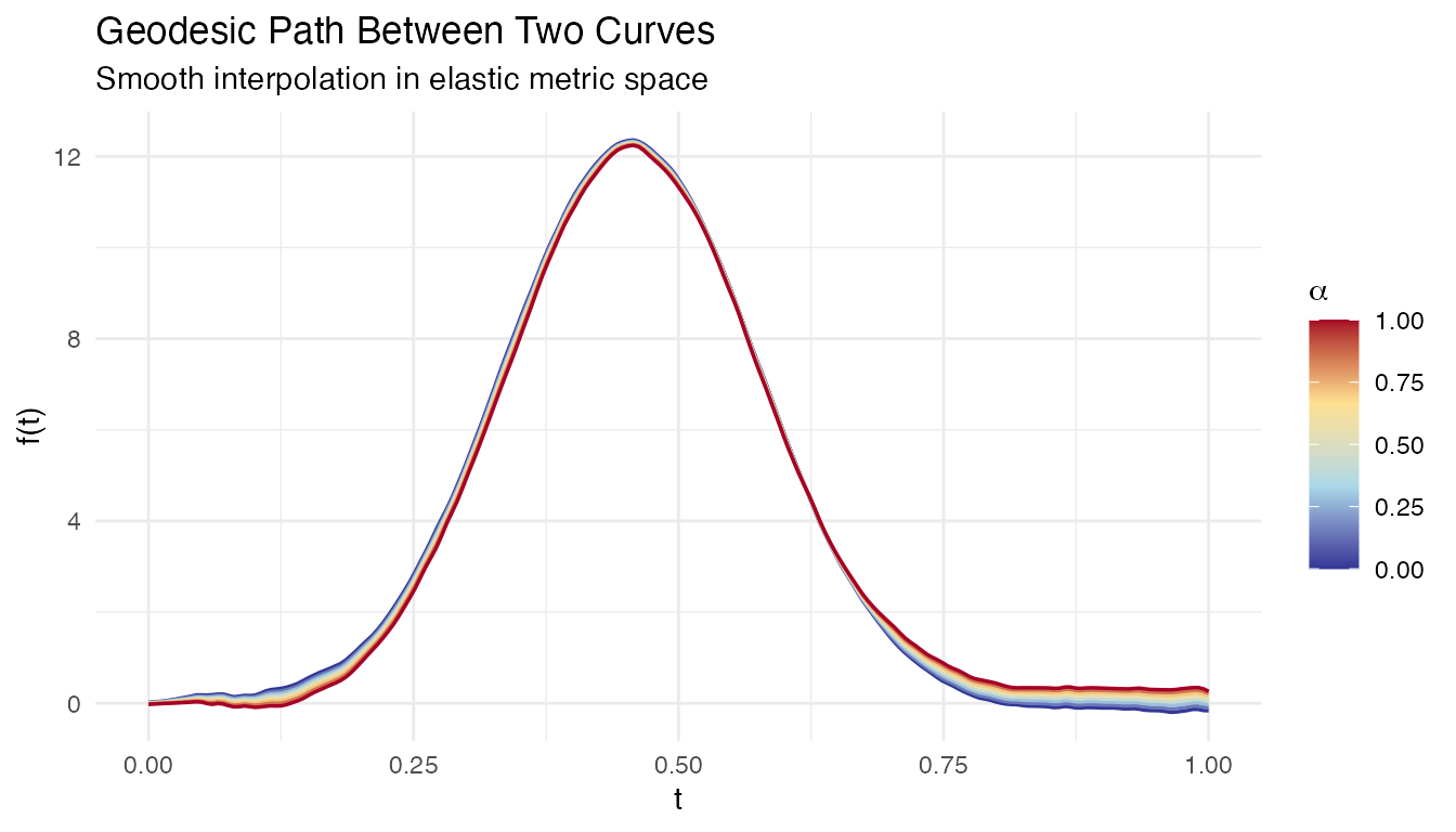

References:

Srivastava, A. & Klassen, E. P. (2016). Functional and Shape Data Analysis. Springer. Chapter 4: Elastic Shape Analysis of Curves.
Srivastava, A., Klassen, E., Joshi, S. H., & Jermyn, I. H. (2011). Shape analysis of elastic curves in Euclidean spaces. IEEE TPAMI, 33(7), 1415–1428.

11. Gaussian Generative Model

Motivation

After separating amplitude and phase variability via FPCA, we can build a generative model that synthesizes new curves by sampling from the estimated amplitude and phase distributions. This is useful for data augmentation, simulation studies, and testing.

Method

The generative model fits Gaussian distributions to the vertical (amplitude) and horizontal (phase) FPC scores separately:

Align curves to the Karcher mean and compute vertical FPCA on aligned curves and horizontal FPCA on warping functions
Fit $\mathbf{z}_V \sim N(\mathbf{0}, \Lambda_V)$ to amplitude scores and $\mathbf{z}_H \sim N(\mathbf{0}, \Lambda_H)$ to phase scores
Generate new curves by sampling scores and reconstructing: $f_{\text{new}} = \bar{f} + \sum_k z_{V,k} \xi_k$ warped by $\gamma_{\text{new}} = \text{exp}(\sum_k z_{H,k} \psi_k)$

The joint model preserves amplitude-phase correlations by fitting a joint Gaussian to the concatenated score vectors.

# Fit generative model from Karcher mean result
gm <- gauss.model(km, n.components = 3, n.samples = 20)

cat("Generated", nrow(gm$samples$data), "synthetic curves\n")
#> Generated 20 synthetic curves

# Plot original vs generated
df_gen <- rbind(
  data.frame(t = rep(t_grid, nrow(fd$data)),
             value = as.vector(t(fd$data)),
             curve = rep(seq_len(nrow(fd$data)), each = length(t_grid)),
             type = "Original"),
  data.frame(t = rep(t_grid, nrow(gm$samples$data)),
             value = as.vector(t(gm$samples$data)),
             curve = rep(seq_len(nrow(gm$samples$data)) + 100, each = length(t_grid)),
             type = "Generated")
)

ggplot(df_gen, aes(x = .data$t, y = .data$value,
                    group = .data$curve, color = .data$type)) +
  geom_line(alpha = 0.3, linewidth = 0.4) +
  scale_color_manual(values = c(Original = "#4A90D9", Generated = "#D55E00")) +
  labs(title = "Gaussian Generative Model: Original vs Synthetic Curves",
       x = "t", y = "f(t)", color = NULL) +
  theme(legend.position = "bottom")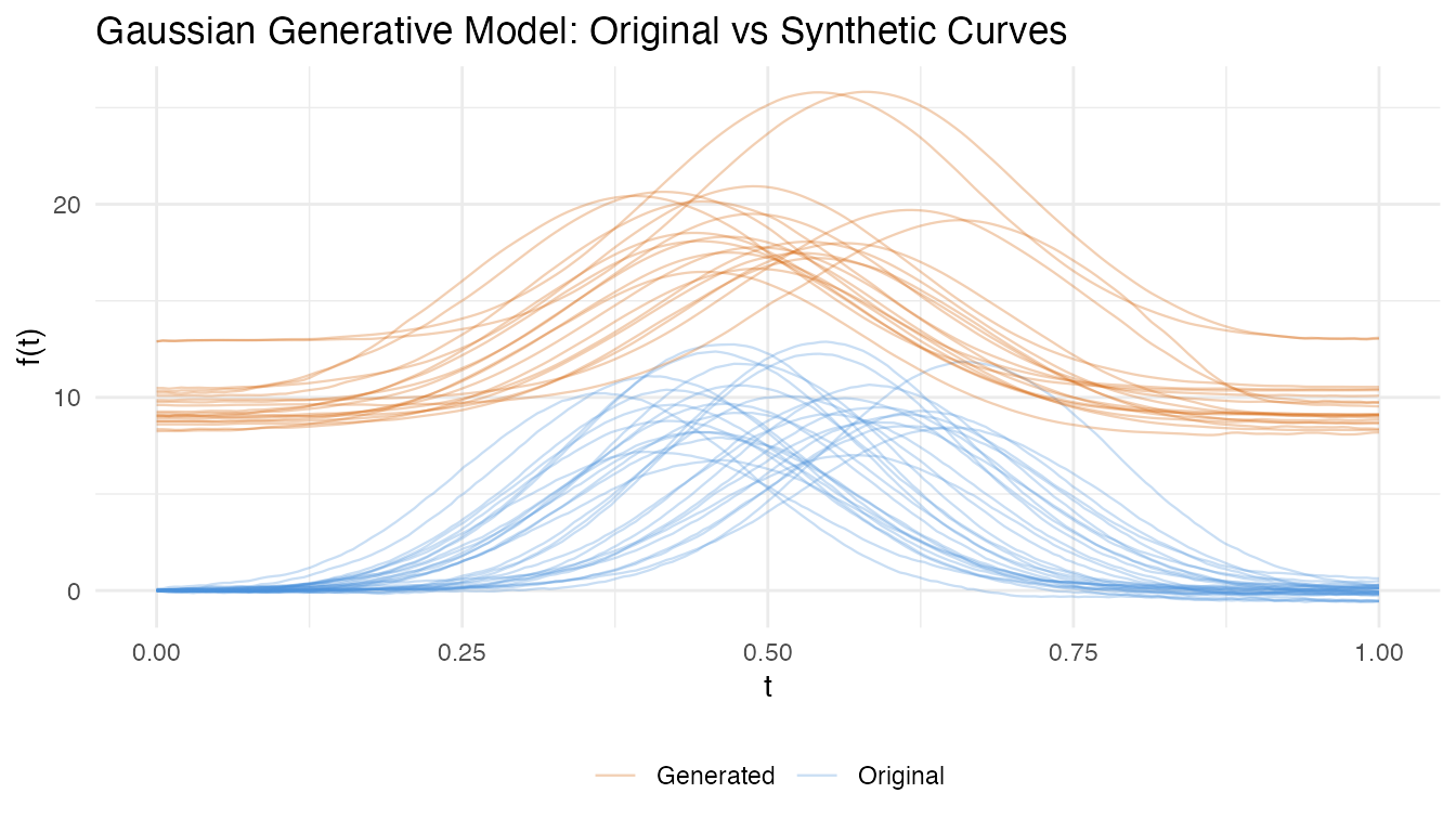

References:

Tucker, J. D., Wu, W., & Srivastava, A. (2013). Generative models for functional data using phase and amplitude separation. Computational Statistics & Data Analysis, 61, 50–66. DOI: 10.1016/j.csda.2012.12.001

12. Peak Persistence Diagram

Motivation

The alignment regularization parameter $\lambda$ controls the trade-off between perfect alignment and smoothness of warping functions. Choosing $\lambda$ is typically ad hoc. Peak persistence provides a topology-based method: by sweeping $\lambda$ from 0 to $\infty$ and tracking when peaks in the Karcher mean appear (“birth”) and disappear (“death”), persistent peaks indicate genuine features while transient peaks indicate noise.

Method

The algorithm computes Karcher means at a grid of $\lambda$ values and builds a persistence diagram:

For each $\lambda$ , compute the Karcher mean $\bar{f}_\lambda$
Detect peaks in $\bar{f}_\lambda$ and track them across $\lambda$ values
A peak is “born” at the $\lambda$ where it first appears and “dies” at the $\lambda$ where it merges with a neighbor
The optimal $\lambda$ is chosen where all persistent peaks are present but noise peaks have died

# Peak persistence diagram for lambda selection
pers <- peak.persistence(fd, lambdas = seq(0, 3, length.out = 15),
                          max.iter = 8)

cat("Optimal lambda:", round(pers$optimal_lambda, 3), "\n")
#> Optimal lambda: 1.5
cat("Peak counts across lambdas:", pers$peak_counts, "\n")
#> Peak counts across lambdas: 0 0 0 0 0 0 0 0 0 0 0 0 0 0 0

References:

Edelsbrunner, H. & Harer, J. (2010). Computational Topology: An Introduction. American Mathematical Society.
Chazal, F., de Silva, V., Glisse, M., & Oudot, S. (2016). The structure and stability of persistence modules. Springer.
Tucker, J. D., Wu, W., & Srivastava, A. (2014). Analysis of proteomics data: phase-amplitude separation using an extended Fisher-Rao metric. Electronic Journal of Statistics, 8, 1724–1733.

13. Horizontal FPNS

Motivation

Standard horizontal FPCA linearizes the space of warping functions (diffeomorphisms) and performs PCA in the tangent space. This linear approximation can be poor when warps are far from the identity. Functional Principal Nested Spheres (FPNS) performs PCA directly on the Hilbert sphere, extracting nonlinear principal directions.

Method

FPNS iteratively extracts principal geodesic directions on the sphere of SRSF-transformed warping functions:

Map warping functions to the Hilbert sphere via $\psi = \sqrt{\dot{\gamma}}$
Find the great circle (geodesic subspace) that maximizes the explained variance of the projected data
Project the data onto this subspace and repeat on the residuals (on the orthogonal subsphere)

This produces nested spheres $S^{d-1} \supset S^{d-2} \supset \cdots$ that capture decreasing levels of phase variability.

# Horizontal FPNS (nonlinear PCA on warping functions)
fpns_result <- horiz.fpns(km, n.components = 3)

cat("Explained variance:", round(fpns_result$explained_variance, 4), "\n")
#> Explained variance: 1e-04 1e-04 1e-04
cat("Score dimensions:", paste(dim(fpns_result$scores), collapse = " x "), "\n")
#> Score dimensions: 30 x 3

References:

Jung, S., Dryden, I. L., & Marron, J. S. (2012). Analysis of principal nested spheres. Biometrika, 99(3), 551–568. DOI: 10.1093/biomet/ass022
Tucker, J. D. (2014). Functional component analysis and regression using elastic methods. PhD Thesis, Florida State University.

14. Multivariate Curve Alignment

Motivation

When curves are vector-valued – e.g., 3D motion trajectories $(x(t), y(t), z(t))$ or multivariate sensor data – alignment must find a single warping function that simultaneously aligns all components. The scalar elastic framework extends naturally by using the multivariate SRSF.

Method

For an $\mathbb{R}^d$ -valued curve $\mathbf{f}(t) = (f_1(t), \ldots, f_d(t))$ , the multivariate SRSF is:

$\mathbf{q}(t) = \frac{\dot{\mathbf{f}}(t)}{\sqrt{\|\dot{\mathbf{f}}(t)\|}}$

The elastic distance and Karcher mean generalize directly. The alignment finds a single $\gamma$ that minimizes:

$\sum_{j=1}^{d} \|q_{1,j} - (q_{2,j} \circ \gamma) \sqrt{\dot{\gamma}}\|^2$

# Multivariate Karcher mean (e.g., for 3D motion data)
# Note: N-D alignment requires FdCurveSet inputs -- R wrappers pending
km_nd <- karcher.mean.nd(fd_nd, max.iter = 20)

# Covariance estimation in the tangent space
cov_nd <- karcher.covariance.nd(fd_nd, km_nd)

# Multivariate elastic PCA
pca_nd <- pca.nd(fd_nd, km_nd, n_components = 3)

References:

Srivastava, A. & Klassen, E. P. (2016). Functional and Shape Data Analysis. Springer. Chapter 5: Shapes of Planar Curves.
Kurtek, S. (2017). A geometric approach to pairwise Bayesian alignment of functional data using importance sampling. Electronic Journal of Statistics, 11(1), 502–531.

Feature Summary

Feature	Use Case	Key Function	Section
Robust Karcher mean	Outlier-contaminated data	`karcher.median`, `robust.karcher.mean`	1
Elastic depth	Centrality with phase awareness	`elastic.depth`	2
SRVF outlier detection	Amplitude/phase outlier classification	`elastic.outlier.detection`	3
Shape confidence intervals	Uncertainty on Karcher mean	`shape.confidence.interval`	4
Bayesian alignment	Posterior over warping functions	`bayesian.align.pair`	5
Multi-resolution alignment	Fast alignment for long curves	`elastic.align.pair.multires`	6
Closed curve alignment	Periodic/closed shapes	`elastic.align.pair.closed`	7
Elastic partial matching	Subsequence search	`elastic.partial.match`	8
Transfer alignment	Cross-population alignment	`transfer.alignment`	9
Curve geodesic	Shape interpolation	`curve.geodesic`	10
Gaussian generative model	Synthetic curve generation	`gauss.model`	11
Peak persistence	Automatic lambda selection	`peak.persistence`	12
Horizontal FPNS	Nonlinear phase PCA	`horiz.fpns`	13
Multivariate alignment	Vector-valued curves	`karcher.mean.nd`	14

References

Srivastava, A. & Klassen, E. P. (2016). Functional and Shape Data Analysis. Springer Series in Statistics. DOI: 10.1007/978-1-4939-4020-2
Srivastava, A., Klassen, E., Joshi, S. H., & Jermyn, I. H. (2011). Shape analysis of elastic curves in Euclidean spaces. IEEE TPAMI, 33(7), 1415–1428.
Tucker, J. D., Wu, W., & Srivastava, A. (2013). Generative models for functional data using phase and amplitude separation. CSDA, 61, 50–66.
Marron, J. S., Ramsay, J. O., Sangalli, L. M., & Srivastava, A. (2015). Functional data analysis of amplitude and phase variation. Statistical Science, 30(4), 468–484. DOI: 10.1214/15-STS524

Introduction

1. Robust Karcher Mean and Median

Motivation

Mathematical Background

2. Elastic Depth

Motivation

Method

3. SRVF Outlier Detection

Motivation

Method

4. Shape Confidence Intervals

Motivation

Method

5. Bayesian Alignment

Motivation

Method

6. Multi-Resolution Alignment

Motivation

Method

7. Closed Curve Alignment

Motivation

Method

8. Elastic Partial Matching

Motivation

Method

9. Transfer Alignment

Motivation

Method

10. Curve Geodesic Interpolation

Motivation

Method

11. Gaussian Generative Model

Motivation

Method

12. Peak Persistence Diagram

Motivation

Method

13. Horizontal FPNS

Motivation

Method

14. Multivariate Curve Alignment

Motivation

Method

Feature Summary

See Also

References