Introduction
When comparing functional data, observed curves often exhibit both amplitude variability (differences in height/shape) and phase variability (differences in timing/speed). Standard methods like the cross-sectional mean or PCA treat all variation as amplitude, which can produce blurred averages and inflated variance.
Elastic alignment separates these two sources of variability by finding optimal warping functions that retime each curve before comparison. The mathematical framework uses the Square-Root Slope Function (SRSF) representation, which makes the Fisher-Rao metric equivalent to the metric – enabling efficient dynamic programming alignment.

Quick Start
set.seed(42)
argvals <- seq(0, 1, length.out = 100)

# Simulate curves with horizontal shifts
n <- 15
shifts <- runif(n, -0.1, 0.1)
data <- matrix(0, n, 100)
for (i in 1:n) {
  data[i, ] <- sin(2 * pi * (argvals - shifts[i]))
}
fd <- fdata(data, argvals = argvals)

# Align to cross-sectional mean (default)
res <- elastic.align(fd)
print(res)
#> Elastic Alignment
#>   Curves: 15 x 100 grid points
#>   Mean elastic distance: 0.2025
plot(res, type = "both")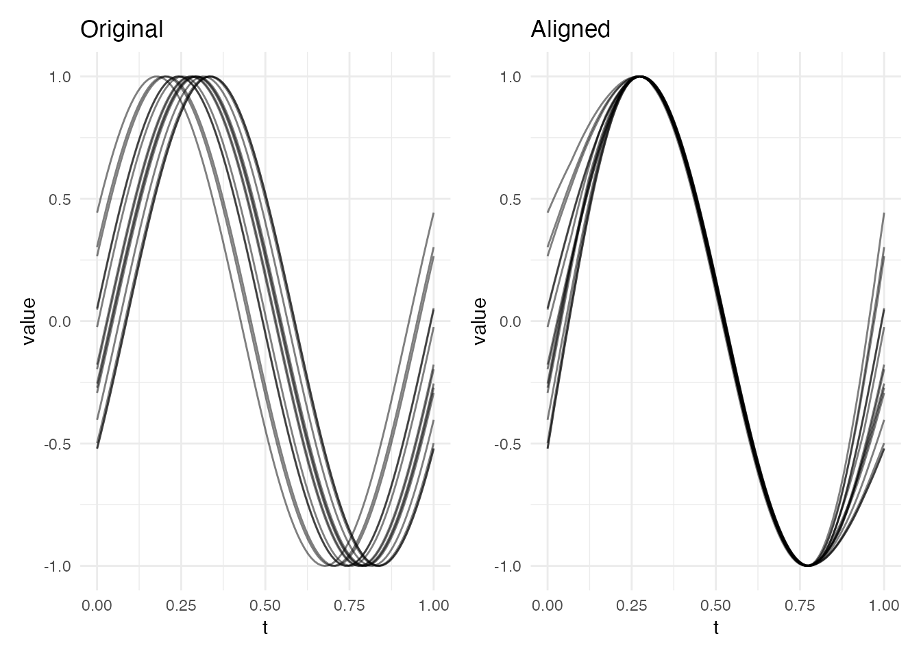
You can also supply a custom target – as a numeric vector or an
fdata object:
# Use the deepest (most central) curve as target
depths <- depth(fd, method = "FM")
res_deep <- elastic.align(fd, target = fd[which.max(depths)])
Inspecting Warping Functions
The warping functions are the key output of elastic alignment. Each is a monotonically increasing function from to that maps the reference time axis to the original curve’s time axis. The aligned curve is then – time is reparameterised so that features line up with the target.
plot(res, type = "warps")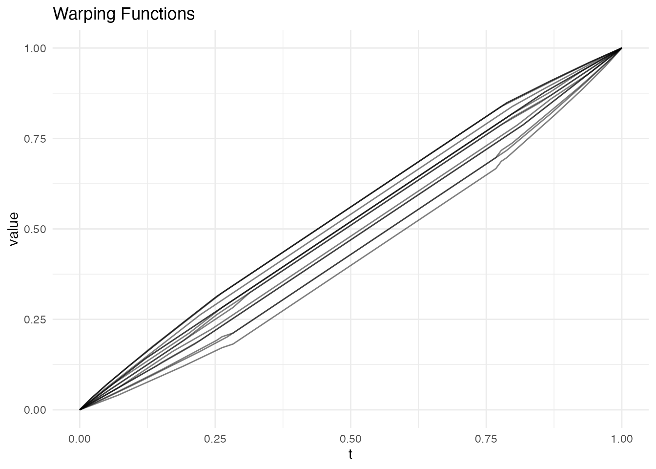
How to Read a Warping Function
The diagonal () represents the identity warp – no time change needed. Deviations from the diagonal tell you how the curve’s timing differs from the reference:
- (below diagonal): at reference time , the corresponding feature in curve occurs at an earlier time. The alignment must look backward to find the matching feature.
- (above diagonal): the feature occurs later in curve . The alignment must look forward.
The slope of encodes local speed:
- (steeper than diagonal): this region of the original curve is stretched – the alignment slows it down to spread features over more reference time.
- (shallower): this region is compressed – the alignment speeds it up.
Let’s visualise this for a single curve to make the interpretation concrete:
# Pick the curve with the largest shift
i_max <- which.max(abs(shifts))
gamma_i <- as.numeric(res$gammas$data[i_max, ])

# Panel 1: the warping function with annotations
df_warp <- data.frame(t = argvals, gamma = gamma_i)
df_diag <- data.frame(t = c(0, 1), gamma = c(0, 1))

p_warp <- ggplot(df_warp, aes(x = t, y = gamma)) +
  geom_line(data = df_diag, linetype = "dashed", color = "grey60") +
  geom_line(color = "steelblue", linewidth = 1) +
  geom_ribbon(aes(ymin = pmin(gamma, t), ymax = pmax(gamma, t)),
              fill = "steelblue", alpha = 0.15) +
  labs(title = paste0("Warping function for curve ", i_max,
                      " (shift = ", round(shifts[i_max], 3), ")"),
       x = "Reference time t", y = expression(gamma(t))) +
  coord_equal()

# Panel 2: original curve, aligned curve, and target
f_orig <- as.numeric(fd$data[i_max, ])
f_aligned <- as.numeric(res$aligned$data[i_max, ])
f_target <- as.numeric(res$target)

df_curves <- data.frame(
  t = rep(argvals, 3),
  value = c(f_orig, f_aligned, f_target),
  curve = rep(c("Original", "Aligned", "Target"), each = length(argvals))
)

p_curves <- ggplot(df_curves, aes(x = t, y = value, color = curve,
                                  linetype = curve)) +
  geom_line(linewidth = 0.9) +
  scale_color_manual(values = c(Original = "coral", Aligned = "steelblue",
                                Target = "grey30")) +
  scale_linetype_manual(values = c(Original = "solid", Aligned = "solid",
                                   Target = "dashed")) +
  labs(title = "Effect of warping on the curve",
       x = "t", y = "value", color = NULL, linetype = NULL) +
  theme(legend.position = "top")

# Panel 3: local speed via deriv()
warp_speed <- deriv(res$gammas)
speed_i <- as.numeric(warp_speed$data[i_max, ])
df_speed <- data.frame(t = warp_speed$argvals, speed = speed_i)

p_speed <- ggplot(df_speed, aes(x = t, y = speed)) +
  geom_hline(yintercept = 1, linetype = "dashed", color = "grey60") +
  geom_line(color = "steelblue", linewidth = 0.8) +
  geom_ribbon(aes(ymin = 1, ymax = speed), fill = "steelblue", alpha = 0.15) +
  labs(title = "Local warping speed: deriv(res$gammas)",
       x = "t",
       y = expression(dot(gamma)(t))) +
  annotate("text", x = 0.05, y = max(speed_i) * 0.95, label = "stretched",
           hjust = 0, size = 3, color = "grey40") +
  annotate("text", x = 0.05, y = min(speed_i) * 1.05, label = "compressed",
           hjust = 0, size = 3, color = "grey40")

p_warp / p_curves / p_speed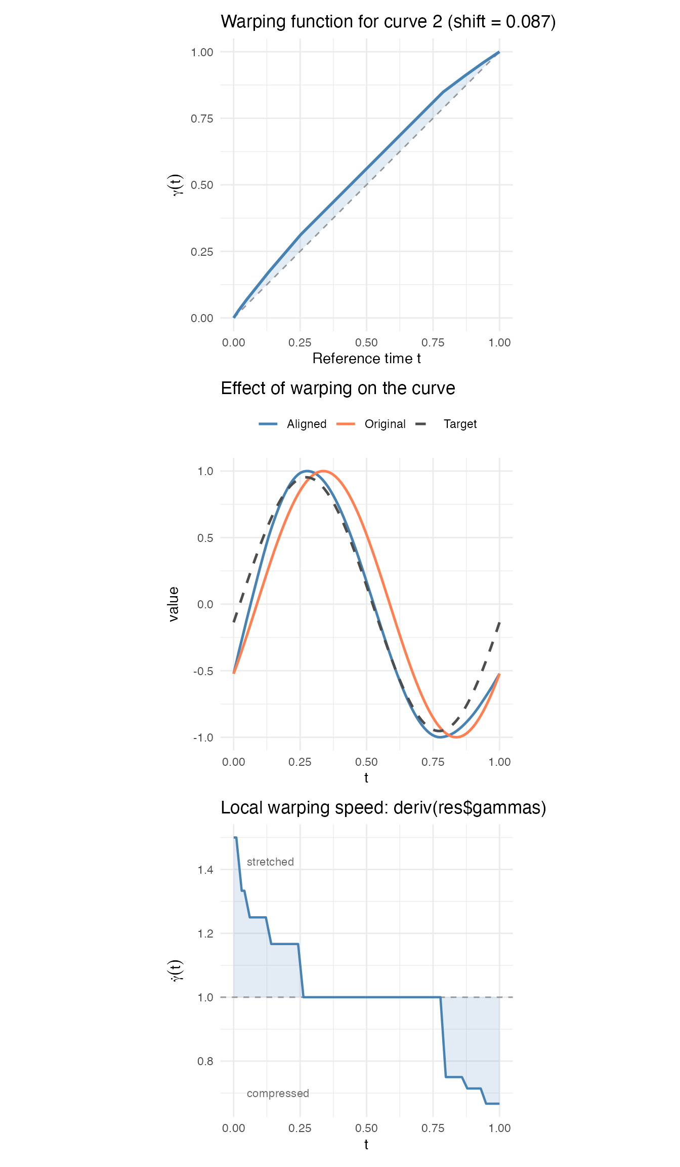
The three panels show the full picture for a single curve:
- Top: the warping function – the shaded area shows deviation from the identity. This curve had a positive shift, so over most of the domain (the alignment needs to look forward to find matching features).
- Middle: the original curve (coral), the target (dashed), and the aligned result (blue). After warping, the aligned curve matches the target closely.
-
Bottom: the local warping speed
,
computed via
deriv(res$gammas). Since the warping functions arefdataobjects,deriv()returns anfdataof derivatives. Where , time is being stretched; where , time is compressed. The regions of fastest change correspond to where the original curve’s features were most offset from the target.
How It Works (Intuition)
Imagine you record the heartbeat signal of several patients. Each heartbeat has the same features – a P wave, a QRS complex, a T wave – but the timing differs from patient to patient. If you simply average the raw signals, the peaks blur out because they don’t line up.
Elastic alignment fixes this by stretching and compressing the time axis of each curve until corresponding features line up. The key insight is to work with the Square-Root Slope Function (SRSF) – a transformed version of the curve that makes the math tractable. In SRSF space, finding the best alignment reduces to a standard dynamic programming problem that can be solved efficiently.
After alignment, variability splits cleanly into two parts:
- Amplitude variability: genuine differences in curve shape (how tall the peaks are, how deep the valleys)
- Phase variability: differences in timing (when the peaks occur)
The Karcher mean is the average curve shape, computed after alignment. Unlike the ordinary mean, it preserves sharp features because the peaks are aligned before averaging.
Mathematical Framework
The Space of Warping Functions
Let denote the space of absolutely continuous functions . The warping group is the set of orientation-preserving diffeomorphisms of :
acts on by composition: for and , the warped function is . This group action reparameterizes the curve without changing its shape – only the speed at which the curve is traversed changes.
The Fisher-Rao Metric
The Fisher-Rao metric on is the unique Riemannian metric (up to scaling) that is invariant under the action of . For two tangent vectors , it is defined as:
This metric is difficult to compute directly because it depends on the derivative of in the denominator. The SRSF transform resolves this by isometrically mapping the Fisher-Rao geometry to a flat space.
SRSF Transform
The Square-Root Slope Function of is defined as:
This transform has three key properties:
- Isometry: The Fisher-Rao distance between and equals the distance between their SRSFs and (after optimal alignment)
- Equivariance: Under the warping action , the SRSF transforms as . This is simply the standard action of on
- Invertibility: Given and an initial value , the original function is recovered by:
q <- srsf.transform(fd)
p1 <- plot(fd) + labs(title = "Original Curves")
p2 <- plot(q) + labs(title = "SRSF Representation")
p1 + p2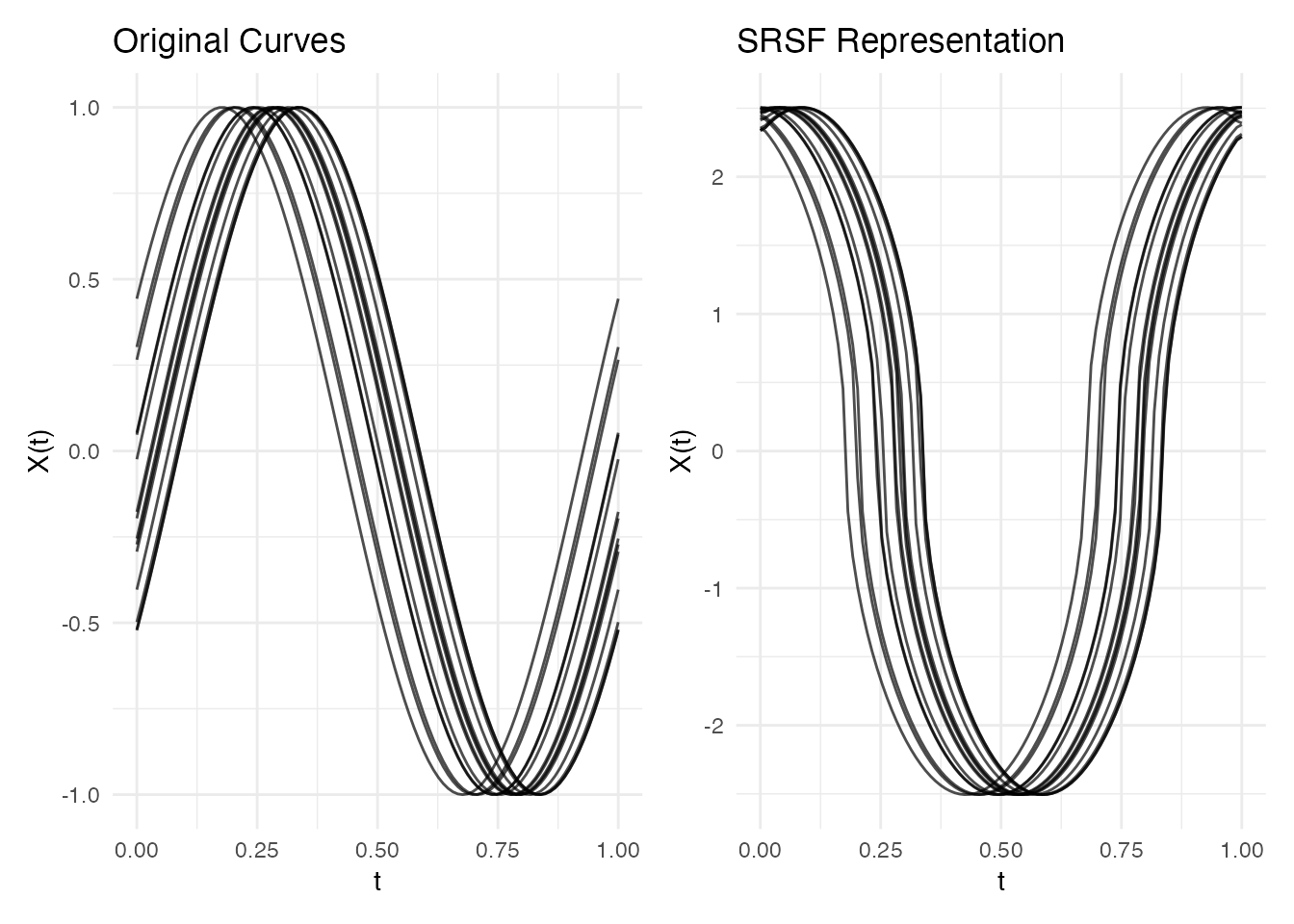
f_original <- fd$data[1, ]
q_values <- q$data[1, ]
f_reconstructed <- srsf.inverse(q_values, argvals, f_original[1])

max_error <- max(abs(f_original - f_reconstructed))
cat("Round-trip max error:", format(max_error, digits = 4), "\n")
#> Round-trip max error: 0.0006717
Alignment as Optimization
Given two functions with SRSFs , the optimal alignment finds:
This is solved via dynamic programming in time, where is the number of grid points. The aligned function is , and the elastic distance between and is:
This distance satisfies all metric axioms (non-negativity, symmetry, triangle inequality) and is invariant to reparameterization: for any .
Amplitude-Phase Decomposition
Elastic alignment provides a principled decomposition of total variability. For a sample with aligned versions :
- Amplitude variability: The residual variance in after alignment. This captures genuine differences in curve shape (height, depth of features)
- Phase variability: The variability in the warping functions themselves. This captures differences in timing (when features occur)
The variance reduction (VR) quantifies the proportion of total variance attributable to phase:
where denotes the mean pointwise variance . A VR close to 1 indicates that most variability was phase (and has been removed); a VR near 0 indicates the variability is primarily amplitude.
Karcher Mean
The Karcher mean (Frechet mean in the elastic metric) is the function that minimizes the sum of squared elastic distances:
Since accounts for reparameterization, is a shape-preserving average: it recovers the common shape without blurring from phase variability. The algorithm iterates:
- Initialize (cross-sectional mean)
- Align all curves to :
- Update
- Repeat until convergence ()
In practice, convergence is guaranteed to a local minimum and typically occurs in 5–20 iterations.
Core Functions
Karcher Mean
km <- karcher.mean(fd, max.iter = 20, tol = 1e-4)
print(km)
#> Karcher Mean (Elastic)
#>   Curves: 15 x 100 grid points
#>   Iterations: 15
#>   Converged: FALSE
cross_mean <- as.numeric(mean(fd)$data)
karcher <- as.numeric(km$mean$data)

df_means <- data.frame(
  t = rep(argvals, 2),
  value = c(cross_mean, karcher),
  type = rep(c("Cross-sectional mean", "Karcher mean"), each = 100)
)

ggplot(df_means, aes(x = t, y = value, color = type)) +
  geom_line(linewidth = 1.2) +
  scale_color_manual(values = c("Cross-sectional mean" = "steelblue",
                                "Karcher mean" = "firebrick")) +
  labs(title = "Cross-Sectional vs Karcher Mean",
       x = "t", y = "f(t)", color = NULL)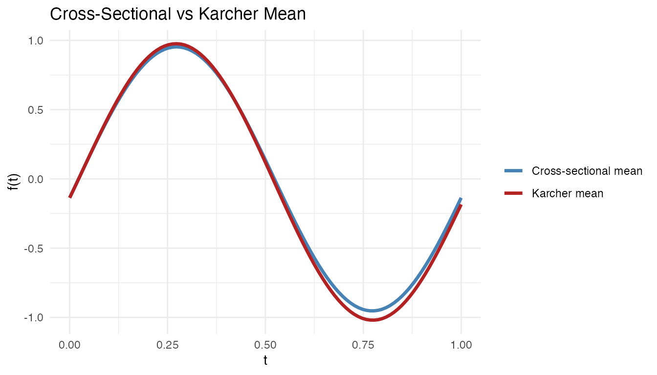
The cross-sectional mean is attenuated by the phase shifts, while the Karcher mean recovers the true amplitude.
For complex data, increase max.iter and check
convergence:
set.seed(42)
n <- 20
dm <- matrix(0, n, 100)
for (i in 1:n) {
  shift <- runif(1, -0.1, 0.1)
  dm[i, ] <- exp(-25 * (argvals - 0.5 - shift)^2)
}
fd_bumps <- fdata(dm, argvals = argvals)

km <- karcher.mean(fd_bumps, max.iter = 30, tol = 1e-4)
cat("Converged:", km$converged, "\n")
#> Converged: FALSE
cat("Iterations:", km$n.iter, "\n")
#> Iterations: 30
plot(km, type = "mean")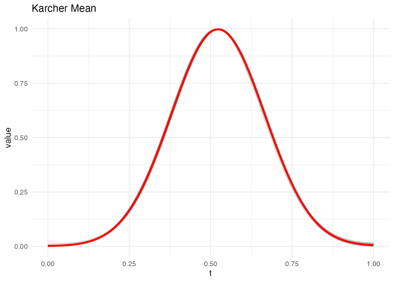
Elastic Distance Matrix
The elastic distance provides a reparameterization-invariant metric for clustering, MDS, and other distance-based methods:
D <- elastic.distance(fd)

# Metric properties
cat("Symmetric:             ", max(abs(D - t(D))) < 1e-10, "\n")
#> Symmetric:              TRUE
cat("Non-negative:          ", all(D >= -1e-10), "\n")
#> Non-negative:           TRUE
cat("Zero diagonal:         ", all(abs(diag(D)) < 1e-10), "\n")
#> Zero diagonal:          TRUE
mds <- cmdscale(D, k = 2)
plot(mds, pch = 19, xlab = "MDS 1", ylab = "MDS 2",
     main = "MDS of Elastic Distances", col = "steelblue", cex = 1.3)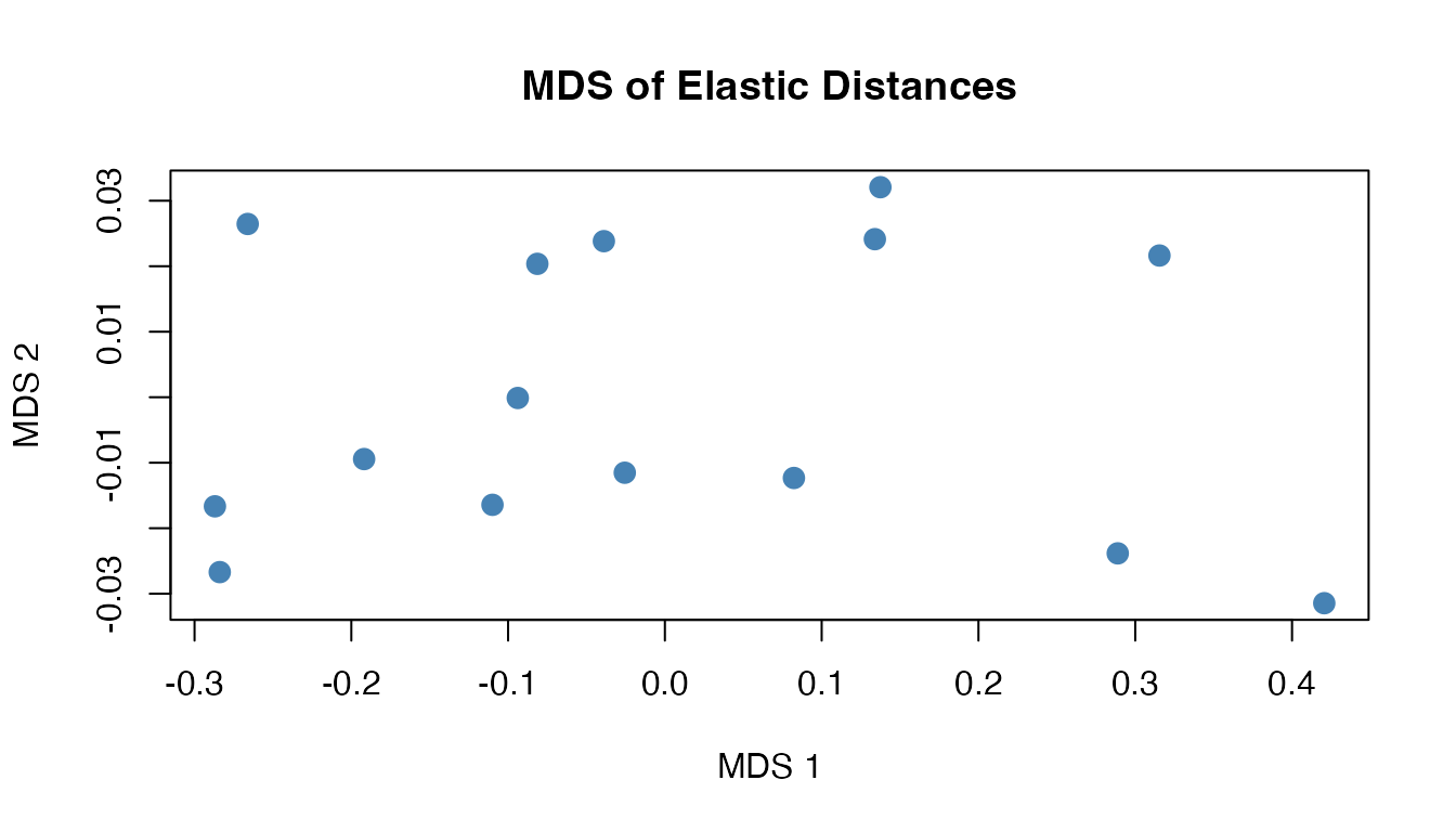
The elastic distance is also available through the
metric() dispatcher:
Amplitude and Phase Distances
The elastic framework uniquely decomposes the total distance between two curves into amplitude (shape) and phase (timing) components:
D_amp <- amplitude.distance(fd, lambda = 0)
D_phase <- phase.distance(fd, lambda = 0)

cat("Amplitude distance (curves 1-2):", round(as.matrix(D_amp)[1, 2], 3), "\n")
#> Amplitude distance (curves 1-2): 0.061
cat("Phase distance (curves 1-2):    ", round(as.matrix(D_phase)[1, 2], 3), "\n")
#> Phase distance (curves 1-2):     0.051
cat("Elastic distance (curves 1-2):  ", round(D[1, 2], 3), "\n")
#> Elastic distance (curves 1-2):   0.061
For these phase-shifted sine curves, most of the distance comes from phase (timing differences), with very little amplitude distance (the shapes are similar after alignment).
Alignment Quality Diagnostics
After alignment, we can quantify exactly what changed. First, compute the Karcher mean and alignment quality:
km_diag <- karcher.mean(fd, max.iter = 20, tol = 1e-4)
aq <- alignment.quality(fd, km_diag)
print(aq)
#> Alignment Quality Diagnostics
#>   Mean warp complexity: 0.0666
#>   Mean warp smoothness: 19.2674
#>   Total variance:      0.0457
#>   Amplitude variance:  0.0104
#>   Phase variance:      0.0353
#>   Phase/Total ratio:   0.7725
#>   Mean VR:             0.1483
Before vs After: What Changed?
To see the effect of alignment concretely, we compare key metrics computed on the original and aligned curves:
# Pairwise L2 distances
D_before <- as.matrix(metric.lp(fd))
D_after <- as.matrix(metric.lp(km_diag$aligned))
mean_d_before <- mean(D_before[upper.tri(D_before)])
mean_d_after <- mean(D_after[upper.tri(D_after)])

# Pointwise variance
var_before <- apply(fd$data, 2, var)
var_after <- apply(km_diag$aligned$data, 2, var)
mean_var_before <- mean(var_before)
mean_var_after <- mean(var_after)

# Format as table
pct <- function(b, a) paste0(round((b - a) / b * 100, 1), "%")
tab <- data.frame(
  Metric = c("Mean pairwise L\u00b2 distance",
             "Mean pointwise variance",
             "Mean cross-sectional SD"),
  Before = round(c(mean_d_before, mean_var_before, mean(sqrt(var_before))), 4),
  After = round(c(mean_d_after, mean_var_after, mean(sqrt(var_after))), 4),
  Reduction = c(pct(mean_d_before, mean_d_after),
                pct(mean_var_before, mean_var_after),
                pct(mean(sqrt(var_before)), mean(sqrt(var_after))))
)
knitr::kable(tab, align = "lrrr")| Metric | Before | After | Reduction |
|---|---|---|---|
| Mean pairwise L² distance | 0.2603 | 0.1242 | 52.3% |
| Mean pointwise variance | 0.0494 | 0.0120 | 75.7% |
| Mean cross-sectional SD | 0.2043 | 0.0646 | 68.4% |
Pointwise Variance: Where Did Alignment Help?
The pointwise variance at each time point shows where alignment had the greatest effect. The shaded region highlights the variance removed:
df_var <- data.frame(
  t = rep(argvals, 2),
  variance = c(var_before, var_after),
  stage = rep(c("Before", "After"), each = length(argvals))
)

ggplot() +
  geom_ribbon(
    data = data.frame(t = argvals, ymin = var_after, ymax = var_before),
    aes(x = t, ymin = ymin, ymax = ymax),
    fill = "steelblue", alpha = 0.2
  ) +
  geom_line(data = df_var,
            aes(x = t, y = variance, color = stage, linetype = stage),
            linewidth = 0.8) +
  scale_color_manual(values = c(Before = "grey40", After = "steelblue")) +
  scale_linetype_manual(values = c(Before = "dashed", After = "solid")) +
  labs(title = "Pointwise Variance: Before vs After Alignment",
       x = "t", y = "Variance", color = NULL, linetype = NULL) +
  theme(legend.position = "top")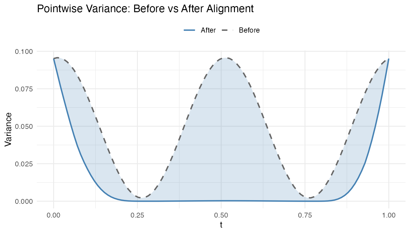
Mean Curve: How Does the Average Sharpen?
The cross-sectional mean of the original curves is blurred by timing differences. The Karcher mean, computed after alignment, recovers a sharper representative shape:
n <- nrow(fd$data)
m <- ncol(fd$data)

# Original curves + cross-sectional mean
df_orig <- data.frame(
  t = rep(argvals, n), value = as.vector(t(fd$data)),
  curve = rep(seq_len(n), each = m)
)
cross_mean <- as.numeric(mean(fd)$data)
df_cmean <- data.frame(t = argvals, value = cross_mean)

p1 <- ggplot() +
  geom_line(data = df_orig, aes(x = t, y = value, group = curve),
            alpha = 0.15, color = "grey50") +
  geom_line(data = df_cmean, aes(x = t, y = value),
            color = "coral", linewidth = 1.2) +
  labs(title = "Before: Cross-Sectional Mean", x = "t", y = "value")

# Aligned curves + Karcher mean
df_aln <- data.frame(
  t = rep(argvals, n), value = as.vector(t(km_diag$aligned$data)),
  curve = rep(seq_len(n), each = m)
)
df_kmean <- data.frame(t = argvals, value = as.numeric(km_diag$mean$data[1, ]))

p2 <- ggplot() +
  geom_line(data = df_aln, aes(x = t, y = value, group = curve),
            alpha = 0.15, color = "grey50") +
  geom_line(data = df_kmean, aes(x = t, y = value),
            color = "steelblue", linewidth = 1.2) +
  labs(title = "After: Karcher Mean", x = "t", y = "value")

p1 + p2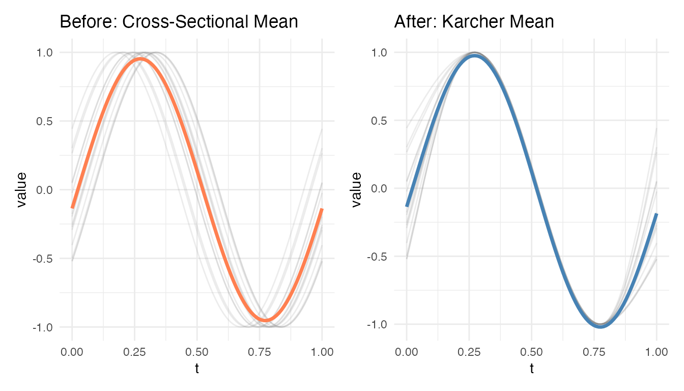
Variance Decomposition
The alignment.quality() result decomposes total variance
into amplitude (shape) and phase (timing) components:
- Variance reduction: fraction of total pointwise variance removed by alignment
- Phase-amplitude ratio: how much of the total variability was due to phase
- Warp complexity: average deviation of warping functions from the identity (higher = more warping needed)
- Warp smoothness: measures the regularity of the warping functions
plot(aq, type = "variance")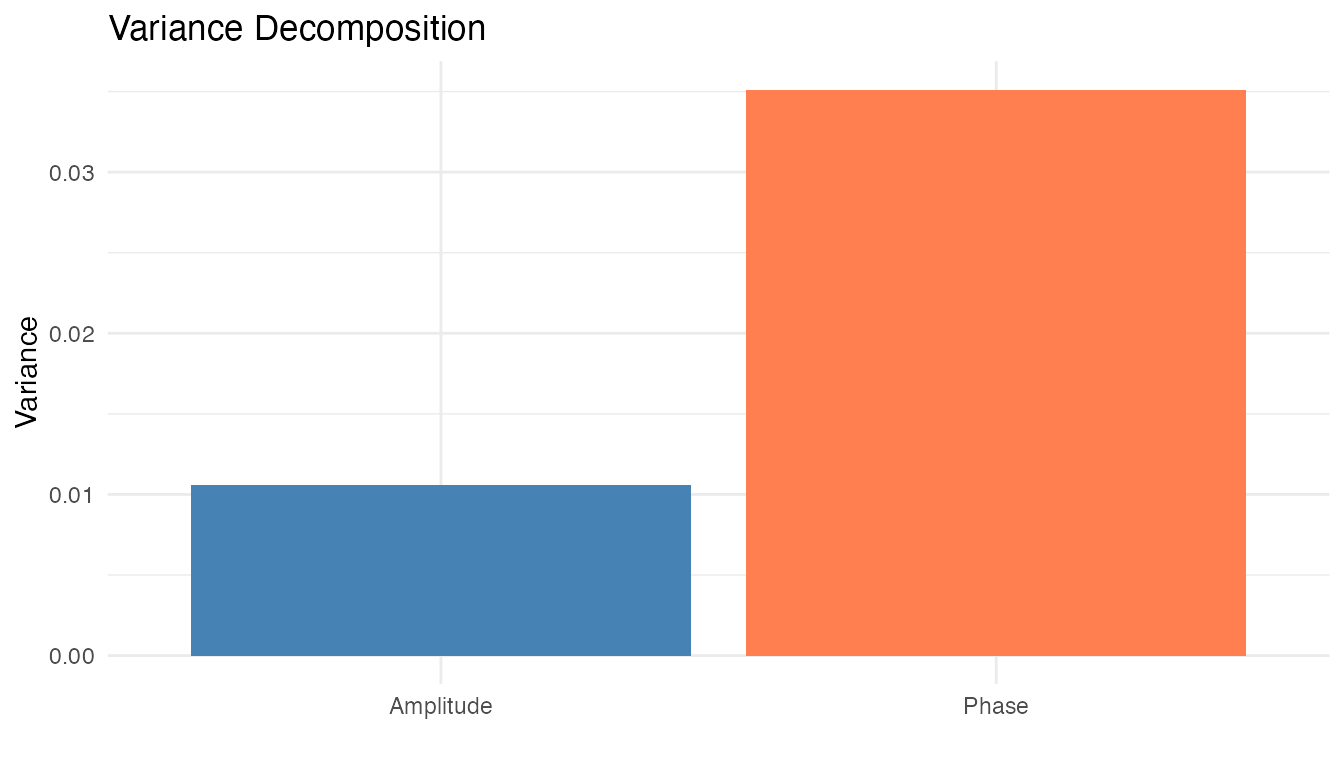
Pairwise Consistency
The alignment.pairwise.consistency() function checks
whether pairwise alignments are consistent – i.e., whether aligning A to
C directly gives the same result as aligning A to B then B to C. A value
near 1 indicates high consistency:
pc <- alignment.pairwise.consistency(fd, lambda = 0, max.triplets = 100)
cat("Pairwise consistency:", round(pc, 3), "\n")
#> Pairwise consistency: 0.004
Low consistency can indicate that the data contains subgroups with different shapes, or that the alignment is sensitive to the choice of target.
Amplitude-Phase Decomposition
For individual curve pairs, elastic.decomposition()
provides the full decomposition of the elastic distance into amplitude
and phase components:
f1 <- fd[1]
f2 <- fd[5]

decomp <- elastic.decomposition(f1, f2, lambda = 0)
cat("Amplitude distance:", round(decomp$d_amplitude, 4), "\n")
#> Amplitude distance: 0.2483
cat("Phase distance:    ", round(decomp$d_phase, 4), "\n")
#> Phase distance:     0.0789
# Visualize the aligned pair
f1_data <- as.numeric(f1$data)
f2_aligned <- decomp$f_aligned
df_pair <- data.frame(
  t = rep(argvals, 2),
  value = c(f1_data, f2_aligned),
  curve = rep(c("f1 (target)", "f2 (aligned)"), each = length(argvals))
)
ggplot(df_pair, aes(x = t, y = value, color = curve)) +
  geom_line(linewidth = 1) +
  scale_color_manual(values = c("f1 (target)" = "steelblue", "f2 (aligned)" = "firebrick")) +
  labs(title = sprintf("Amplitude dist = %.3f, Phase dist = %.3f",
                        decomp$d_amplitude, decomp$d_phase),
       x = "t", y = "f(t)", color = NULL)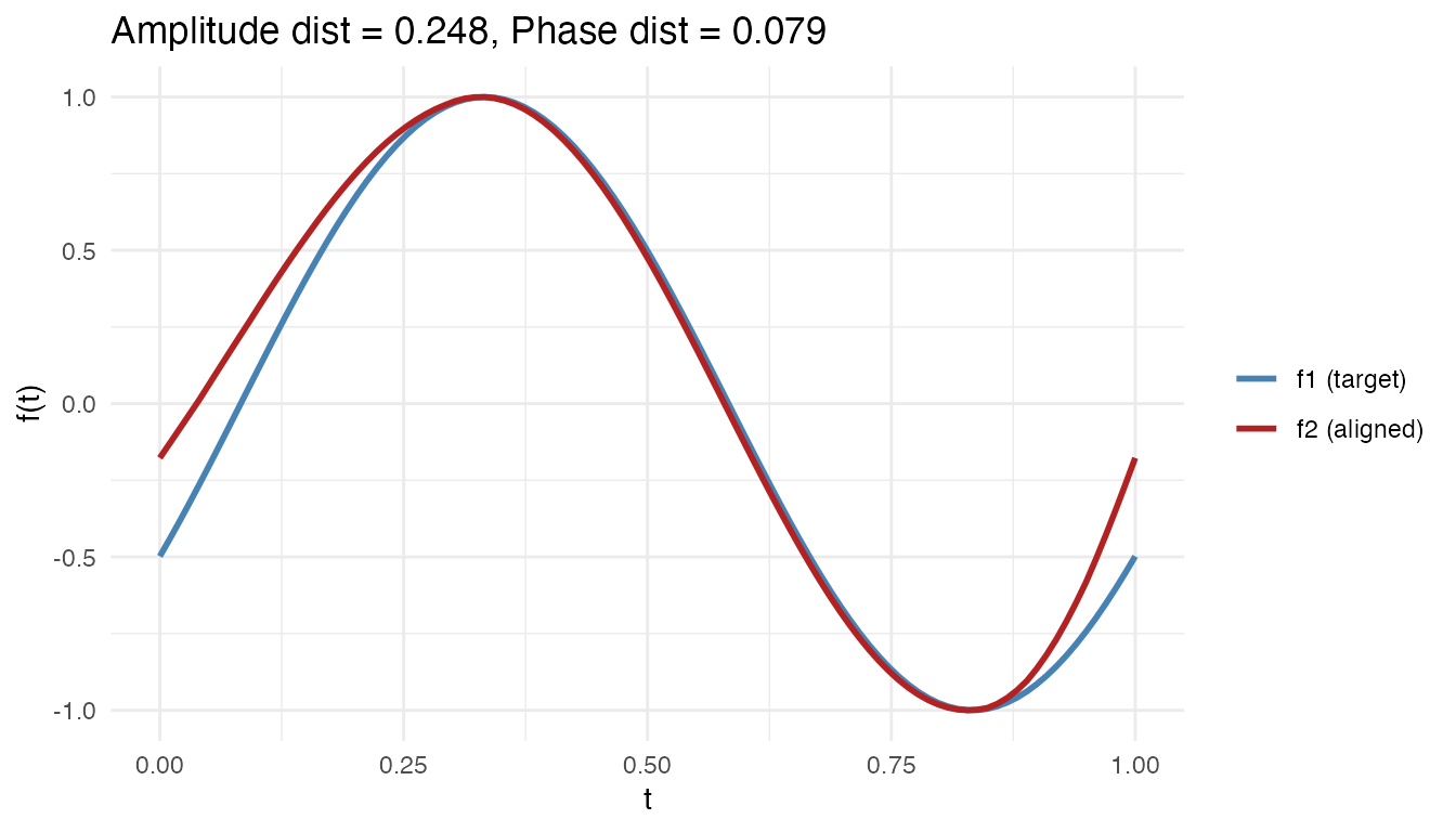
This decomposition is useful for understanding why two curves differ: is it because they have different shapes (amplitude) or different timing (phase)?
Constrained Alignment
When curves have identifiable features (peaks, valleys), you can constrain the elastic alignment to pass through specific landmark positions. This combines the smoothness of elastic warping with guaranteed feature correspondence:
# Detect peaks and constrain alignment to pass through them
ec <- elastic.align.constrained(fd, kind = "peak", min.prominence = 0.3,
                                 expected.count = 1)
p1 <- plot(res, type = "warps") + labs(title = "Elastic Warps")
p2 <- plot(ec, type = "warps") + labs(title = "Constrained Warps")
p1 + p2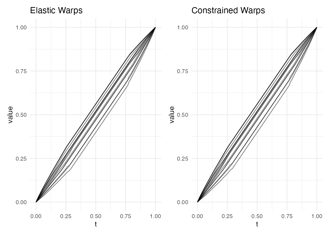
The constrained warps are smooth between landmarks (like elastic) but
anchored at the peak positions (like landmark registration). For a
detailed comparison of all alignment methods, see
vignette("alignment-comparison", package = "fdars").
When to Use Elastic Alignment
Elastic alignment works best when curves share the same shape but differ in timing. The table below summarizes where it excels and where it does not.
Works Well
| Scenario | Typical VR | Notes |
|---|---|---|
| Shifted peaks / bumps | 98-100% | Best case: localized features with horizontal shifts |
| ECG-like sharp peaks | 98-100% | Localized timing differences in multi-peak curves |
| Spectral data (shifted peaks) | 95-98% | Multiple peaks with coherent timing shifts |
| Phase-shifted smooth curves | 90-93% | Sinusoidal, polynomial, sigmoid curves with shifts |
| Non-periodic curves | 95-100% | Works well when boundary values are similar |
Where It Degrades
| Scenario | Typical VR | Explanation |
|---|---|---|
| Mixed amplitude + phase | 40-65% | Phase correction is partial when amplitude dominates |
| Noisy data (raw) | 0-30% | Noise in derivatives overwhelms SRSF; smooth first |
| Large boundary mismatch | 70-85% | Fixed boundary (, ) can’t correct endpoint values |
| Coarse grids (m < 50) | 70-75% | DP resolution limits alignment accuracy |
Where It Should NOT Be Used
| Scenario | What happens | Recommendation |
|---|---|---|
| Pure amplitude differences | Identity warp (no harm, no help) | Use standard methods |
| Rate-varying monotone curves | Spurious warping, VR < 0 | These are amplitude/shape differences, not phase |
| Genuinely different shapes | Forced warping, VR < 0 | Use depth or distance methods instead |
| Very noisy data (unsmoothed) | Noise-driven warping, VR < 0 | Pre-smooth with fdata2basis() +
basis2fdata()
|
Scenario Gallery
The following examples illustrate alignment behavior across different data scenarios. Each shows the original curves (left) and aligned curves (right) with variance reduction (VR) reported.
ECG-like Multi-Peak Curves
Sharp, localized features with timing differences are the ideal use case:
set.seed(42)
n <- 20
dm <- matrix(0, n, 100)
for (i in 1:n) {
  shift <- runif(1, -0.05, 0.05)
  t_shifted <- argvals - shift
  # P wave, QRS complex, T wave
  dm[i, ] <- 0.2 * exp(-200 * (t_shifted - 0.2)^2) -
             0.6 * exp(-500 * (t_shifted - 0.4)^2) +
             1.0 * exp(-800 * (t_shifted - 0.43)^2) -
             0.2 * exp(-500 * (t_shifted - 0.46)^2) +
             0.3 * exp(-150 * (t_shifted - 0.65)^2)
}
fd_ecg <- fdata(dm, argvals = argvals)
res_ecg <- elastic.align(fd_ecg)
vr <- 1 - mean(apply(res_ecg$aligned$data, 2, var)) /
          mean(apply(fd_ecg$data, 2, var))
cat("ECG alignment VR:", round(vr * 100, 1), "%\n")
#> ECG alignment VR: 99.5 %
plot(res_ecg, type = "both")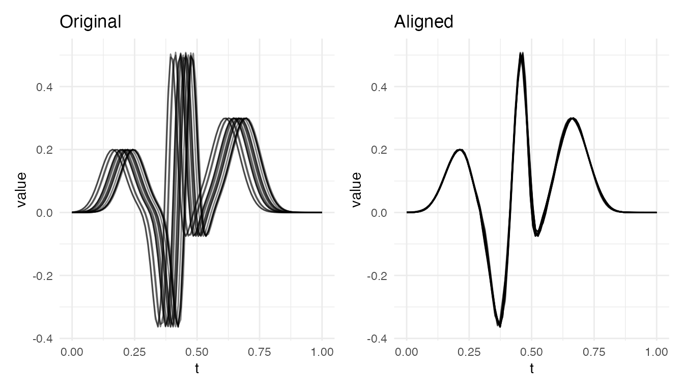
Spectral Peaks
Multiple peaks at varying positions, common in spectroscopy and chromatography:
set.seed(42)
n <- 20
dm <- matrix(0, n, 100)
for (i in 1:n) {
  shift <- runif(1, -0.04, 0.04)
  dm[i, ] <- 0.8 * exp(-300 * (argvals - 0.25 - shift)^2) +
             1.0 * exp(-500 * (argvals - 0.50 - shift * 1.2)^2) +
             0.5 * exp(-300 * (argvals - 0.75 - shift * 0.8)^2)
}
fd_spec <- fdata(dm, argvals = argvals)
res_spec <- elastic.align(fd_spec)
vr <- 1 - mean(apply(res_spec$aligned$data, 2, var)) /
          mean(apply(fd_spec$data, 2, var))
cat("Spectral alignment VR:", round(vr * 100, 1), "%\n")
#> Spectral alignment VR: 99.4 %
plot(res_spec, type = "both")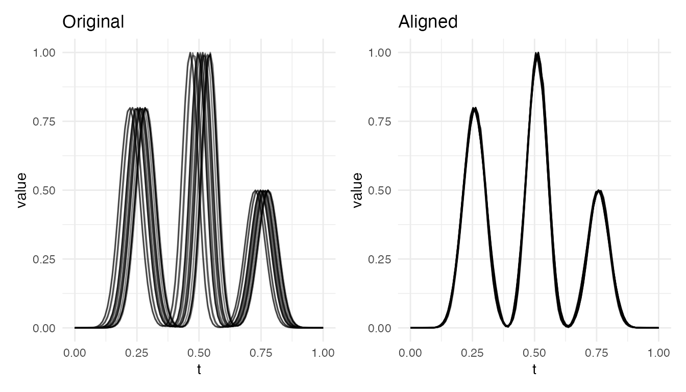
Growth-like Sigmoid Curves
Monotone S-shaped curves with timing shifts (e.g., growth curves with differing onset times):
set.seed(42)
n <- 20
dm <- matrix(0, n, 100)
for (i in 1:n) {
  shift <- runif(1, -0.1, 0.1)
  dm[i, ] <- 1 / (1 + exp(-20 * (argvals - 0.5 - shift)))
}
fd_sig <- fdata(dm, argvals = argvals)
res_sig <- elastic.align(fd_sig)
vr <- 1 - mean(apply(res_sig$aligned$data, 2, var)) /
          mean(apply(fd_sig$data, 2, var))
cat("Sigmoid alignment VR:", round(vr * 100, 1), "%\n")
#> Sigmoid alignment VR: 100 %
plot(res_sig, type = "both")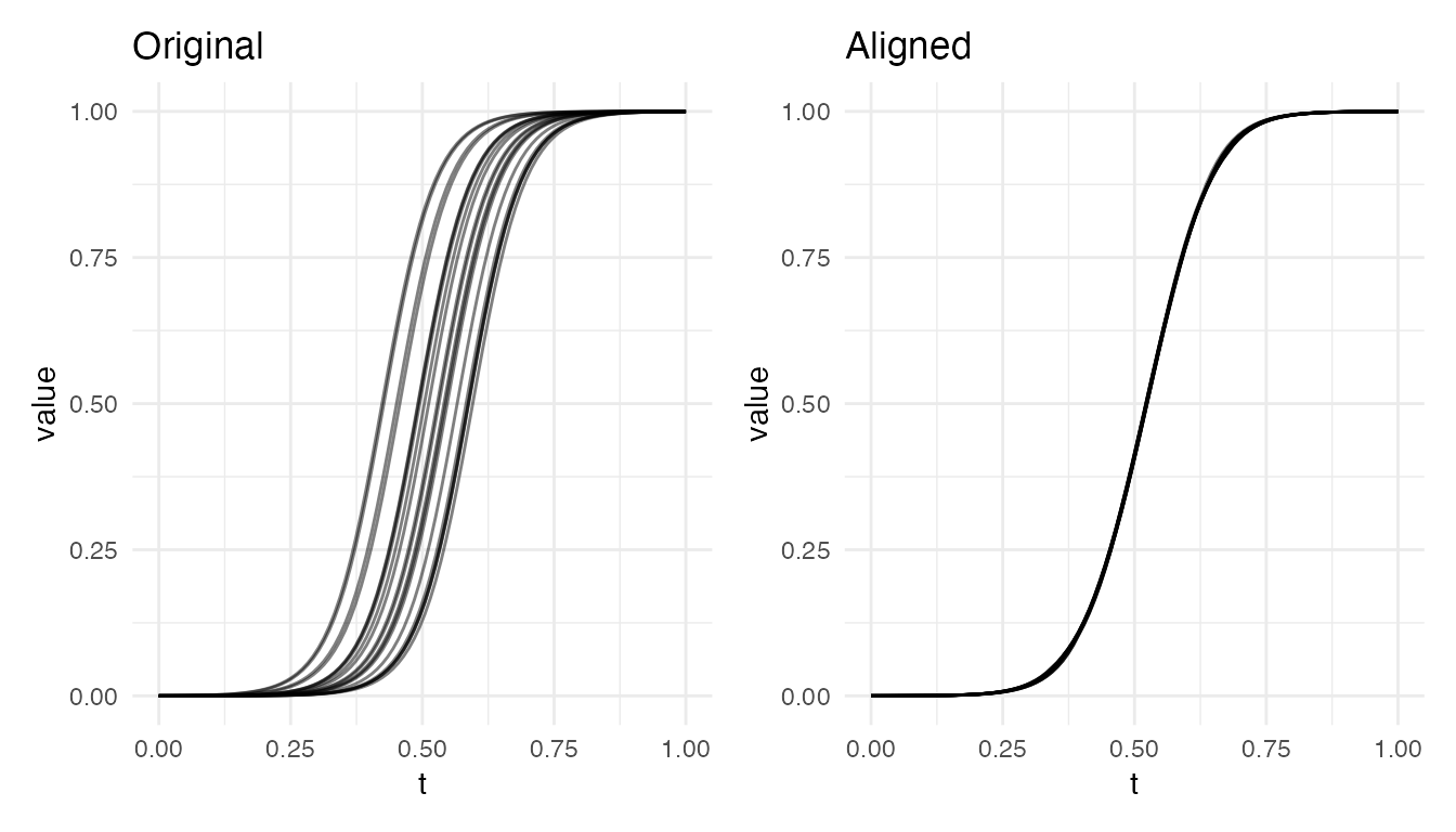
Mixed Amplitude and Phase Variability
When curves differ in both height and timing, alignment corrects the phase component but leaves amplitude variability untouched:
set.seed(42)
n <- 20
dm <- matrix(0, n, 100)
for (i in 1:n) {
  amp <- runif(1, 0.5, 1.5)
  shift <- runif(1, -0.1, 0.1)
  dm[i, ] <- amp * sin(2 * pi * (argvals - shift))
}
fd_mix <- fdata(dm, argvals = argvals)
res_mix <- elastic.align(fd_mix)
vr <- 1 - mean(apply(res_mix$aligned$data, 2, var)) /
          mean(apply(fd_mix$data, 2, var))
cat("Mixed amplitude+phase VR:", round(vr * 100, 1), "%\n")
#> Mixed amplitude+phase VR: 44.4 %
plot(res_mix, type = "both")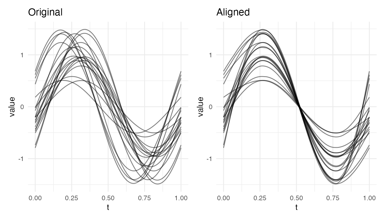
After alignment, curves still differ in amplitude (vertical spread) but peaks and valleys are now synchronized. The residual variance is real amplitude variability, not a failure of alignment.
Noisy Data: Raw vs Smoothed
Noise in derivatives overwhelms the SRSF. Pre-smoothing recovers alignment:
set.seed(42)
n <- 20
dm_clean <- matrix(0, n, 100)
shifts <- runif(n, -0.1, 0.1)
for (i in 1:n) dm_clean[i, ] <- sin(2 * pi * (argvals - shifts[i]))
dm_noisy <- dm_clean + matrix(rnorm(n * 100, sd = 0.3), n, 100)
fd_noisy <- fdata(dm_noisy, argvals = argvals)

# Align raw noisy data
res_noisy <- elastic.align(fd_noisy)
vr_raw <- 1 - mean(apply(res_noisy$aligned$data, 2, var)) /
              mean(apply(fd_noisy$data, 2, var))

# Smooth first, then align
coefs <- fdata2basis(fd_noisy, nbasis = 15, type = "bspline")
fd_sm <- basis2fdata(coefs, argvals)
res_sm <- elastic.align(fd_sm)
vr_sm <- 1 - mean(apply(res_sm$aligned$data, 2, var)) /
             mean(apply(fd_sm$data, 2, var))

cat("Raw VR:     ", round(vr_raw * 100, 1), "%\n")
#> Raw VR:      22.3 %
cat("Smoothed VR:", round(vr_sm * 100, 1), "%\n")
#> Smoothed VR: 66.3 %
plot(res_noisy, type = "both")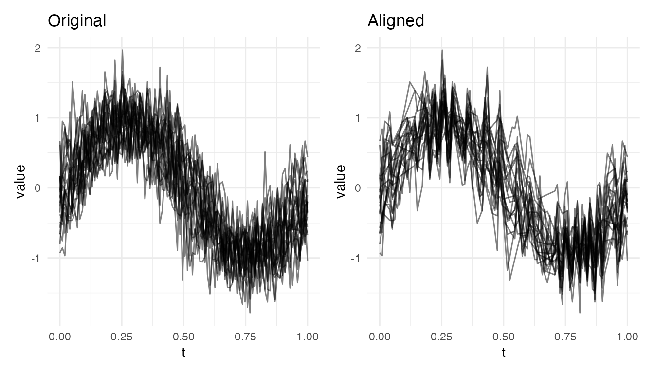
plot(res_sm, type = "both")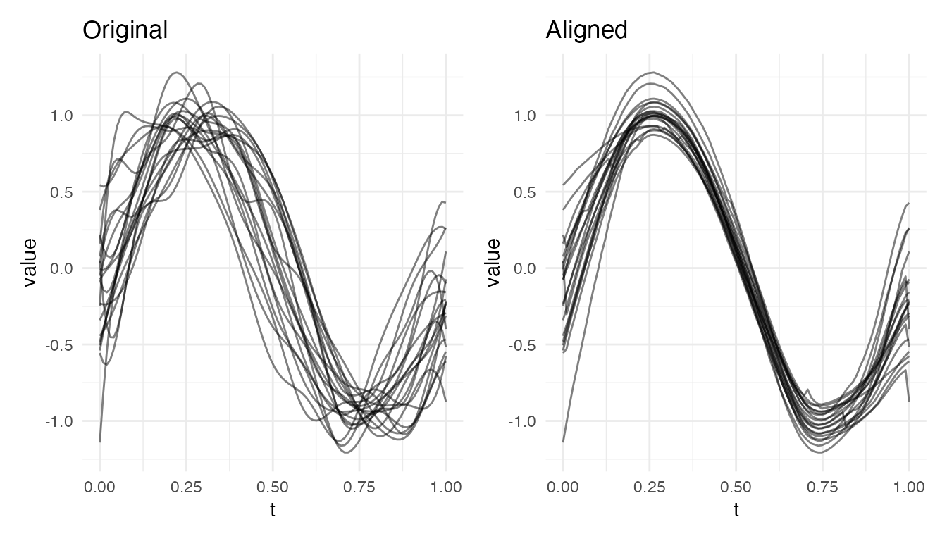
Boundary Mismatch
When shifted curves have different values at the domain boundaries, alignment is excellent in the interior but constrained at the edges:
set.seed(42)
n <- 15
dm <- matrix(0, n, 100)
shifts <- runif(n, -0.15, 0.15)
for (i in 1:n) dm[i, ] <- sin(2 * pi * (argvals - shifts[i]))
fd_bnd <- fdata(dm, argvals = argvals)
res_bnd <- elastic.align(fd_bnd)
vr <- 1 - mean(apply(res_bnd$aligned$data, 2, var)) /
          mean(apply(fd_bnd$data, 2, var))
cat("Boundary mismatch VR:", round(vr * 100, 1), "% — note residual spread at boundaries\n")
#> Boundary mismatch VR: 77 % — note residual spread at boundaries
plot(res_bnd, type = "both")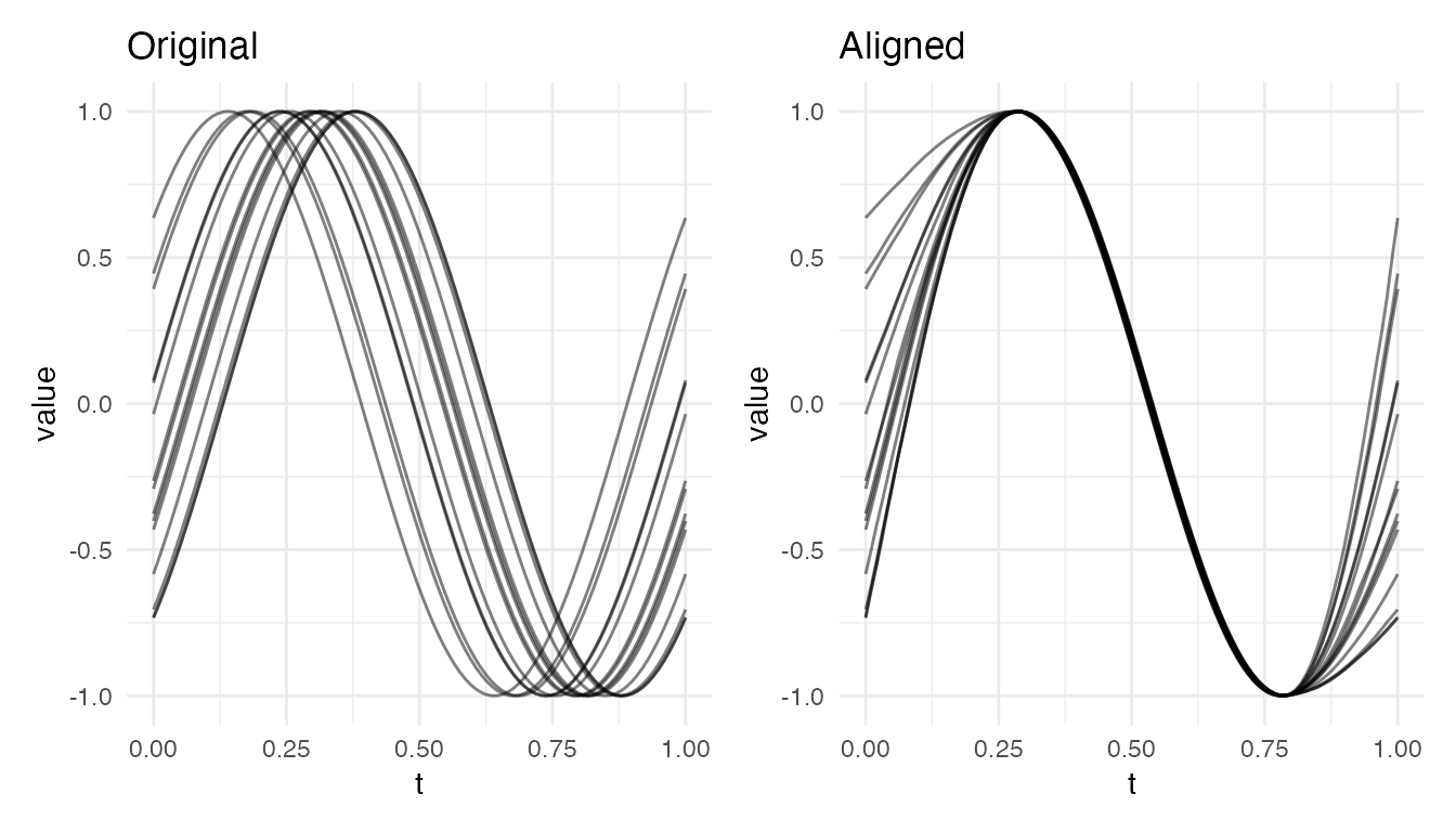
Pure Amplitude Differences
When curves differ only in height (no phase variability), alignment correctly produces identity warps – no benefit, but no harm:
set.seed(42)
n <- 15
dm <- matrix(0, n, 100)
for (i in 1:n) {
  amp <- runif(1, 0.5, 2.0)
  dm[i, ] <- amp * sin(2 * pi * argvals)
}
fd_amp <- fdata(dm, argvals = argvals)
res_amp <- elastic.align(fd_amp)
vr <- 1 - mean(apply(res_amp$aligned$data, 2, var)) /
          mean(apply(fd_amp$data, 2, var))
cat("Pure amplitude VR:", round(vr * 100, 1), "% — identity warps applied\n")
#> Pure amplitude VR: 0 % — identity warps applied
plot(res_amp, type = "both")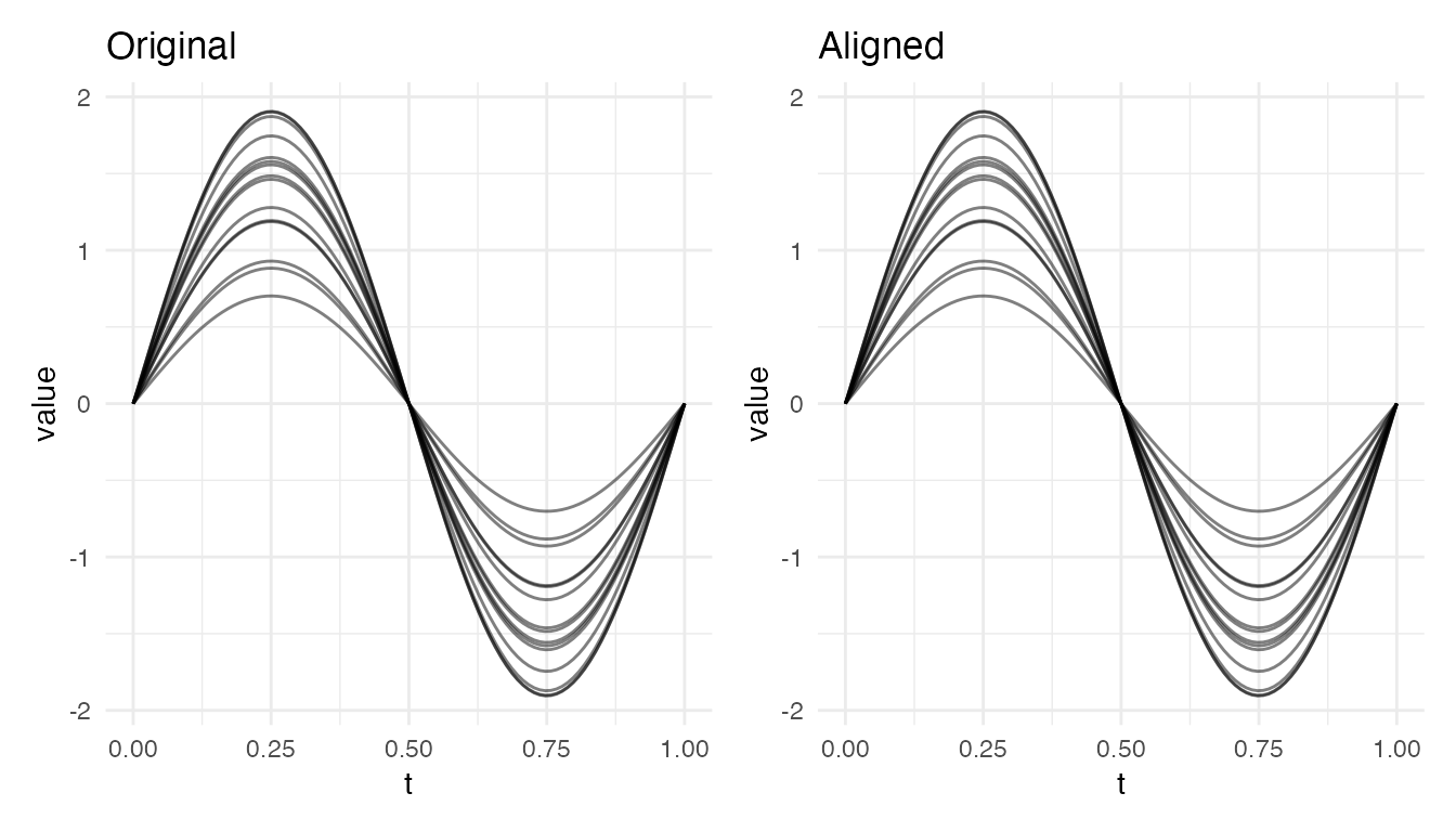
Genuinely Different Shapes
Alignment should not be used when curves have fundamentally different shapes. Forced warping produces meaningless results:
set.seed(42)
n <- 15
dm <- matrix(0, n, 100)
for (i in 1:n) {
  if (i %% 5 == 1) dm[i, ] <- sin(2 * pi * argvals)
  else if (i %% 5 == 2) dm[i, ] <- cos(6 * pi * argvals)
  else if (i %% 5 == 3) dm[i, ] <- argvals^3
  else if (i %% 5 == 4) dm[i, ] <- sin(10 * pi * argvals) * exp(-3 * argvals)
  else dm[i, ] <- dnorm(argvals, 0.5, 0.05) / dnorm(0.5, 0.5, 0.05)
}
fd_diff <- fdata(dm, argvals = argvals)
res_diff <- elastic.align(fd_diff)
vr <- 1 - mean(apply(res_diff$aligned$data, 2, var)) /
          mean(apply(fd_diff$data, 2, var))
cat("Different shapes VR:", round(vr * 100, 1), "% — forced warping of unrelated shapes\n")
#> Different shapes VR: 40.7 % — forced warping of unrelated shapes
plot(res_diff, type = "both")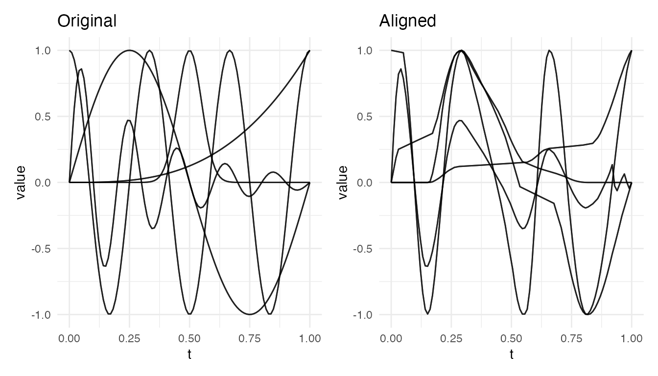
When VR is very low or negative, it indicates the data is not suitable for elastic alignment. Use depth or distance methods instead.
Multi-Bump Scaling
Real-world functional data often contains multiple peaks or features that vary independently. This section explores how elastic alignment handles curves with varying inter-bump distance (peaks shift independently) and varying bump width (peaks broaden or narrow) as the number of bumps increases.
Two Bumps
With two bumps, the warping function has enough freedom to independently adjust each peak’s position and width:
set.seed(42)
m <- 200
argvals_mb <- seq(0, 1, length.out = m)
n <- 20

# Varying inter-bump distance
data_pos <- matrix(0, n, m)
for (i in 1:n) {
  p1 <- 0.3
  p2 <- 0.7 + runif(1, -0.12, 0.12)
  data_pos[i, ] <- exp(-300 * (argvals_mb - p1)^2) +
                   exp(-300 * (argvals_mb - p2)^2)
}
fd_pos <- fdata(data_pos, argvals = argvals_mb)
res_pos <- elastic.align(fd_pos)
vr_pos <- 1 - mean(apply(res_pos$aligned$data, 2, var)) /
              mean(apply(fd_pos$data, 2, var))

# Varying bump width
data_w <- matrix(0, n, m)
for (i in 1:n) {
  w1 <- runif(1, 200, 500)
  w2 <- runif(1, 200, 500)
  data_w[i, ] <- exp(-w1 * (argvals_mb - 0.3)^2) +
                 exp(-w2 * (argvals_mb - 0.7)^2)
}
fd_w <- fdata(data_w, argvals = argvals_mb)
res_w <- elastic.align(fd_w)
vr_w <- 1 - mean(apply(res_w$aligned$data, 2, var)) /
             mean(apply(fd_w$data, 2, var))

cat("2 bumps — varying position: VR =", round(vr_pos * 100, 1), "%\n")
#> 2 bumps — varying position: VR = 100 %
cat("2 bumps — varying width:    VR =", round(vr_w * 100, 1), "%\n")
#> 2 bumps — varying width:    VR = 98.2 %
plot(res_pos, type = "both")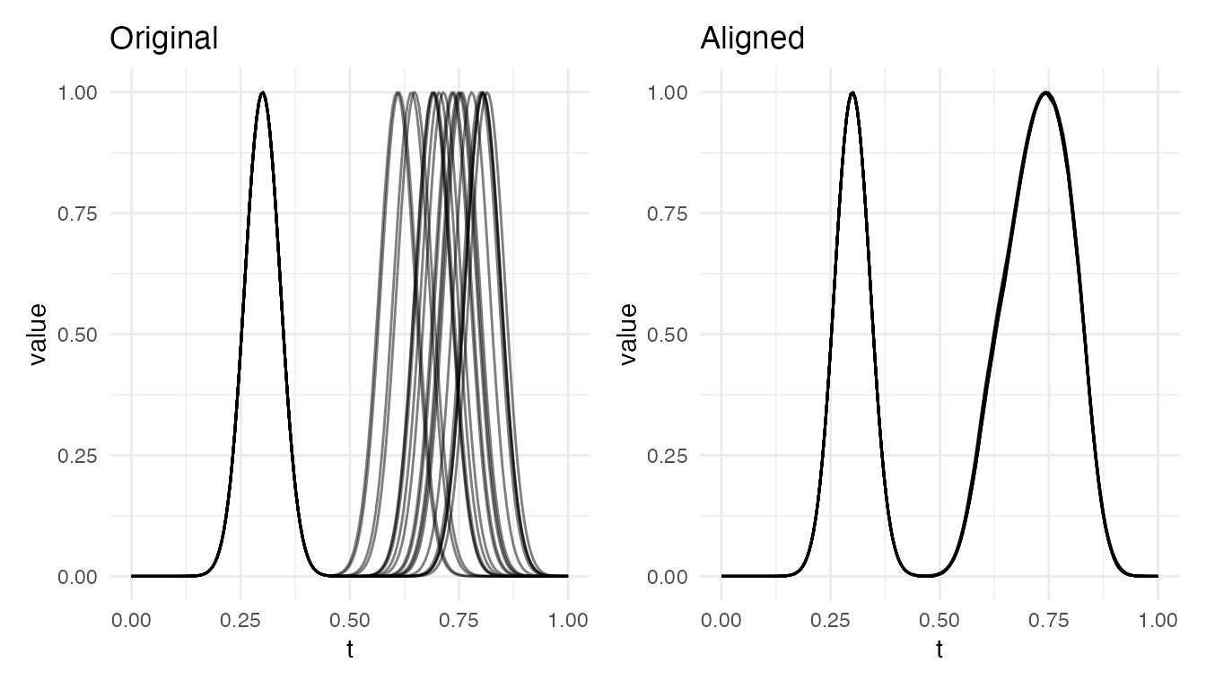
plot(res_w, type = "both")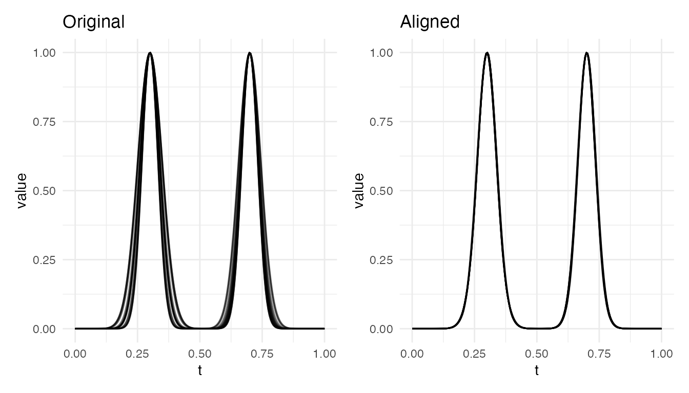
Both cases achieve near-perfect alignment. The warping function locally stretches/compresses the region around each bump to bring peaks into correspondence.
Scaling to More Bumps
As the number of bumps increases, alignment becomes progressively harder. A monotone warping function that stretches one region must compress another, so with many tightly packed bumps the degrees of freedom become insufficient to independently correct each peak.
set.seed(42)
results <- data.frame(
  bumps = integer(), scenario = character(), VR = numeric(),
  stringsAsFactors = FALSE
)

for (nb in c(2, 4, 5, 7)) {
  positions_base <- seq(0.1, 0.9, length.out = nb)

  # Varying positions
  data_pos <- matrix(0, n, m)
  for (i in 1:n) {
    for (j in 1:nb) {
      p <- positions_base[j] + runif(1, -0.04, 0.04)
      data_pos[i, ] <- data_pos[i, ] + exp(-300 * (argvals_mb - p)^2)
    }
  }
  fd_pos <- fdata(data_pos, argvals = argvals_mb)
  res_pos <- elastic.align(fd_pos)
  vr_pos <- 1 - mean(apply(res_pos$aligned$data, 2, var)) /
                mean(apply(fd_pos$data, 2, var))

  # Varying widths
  data_w <- matrix(0, n, m)
  for (i in 1:n) {
    for (j in 1:nb) {
      w <- runif(1, 200, 600)
      data_w[i, ] <- data_w[i, ] + exp(-w * (argvals_mb - positions_base[j])^2)
    }
  }
  fd_w <- fdata(data_w, argvals = argvals_mb)
  res_w <- elastic.align(fd_w)
  vr_w <- 1 - mean(apply(res_w$aligned$data, 2, var)) /
               mean(apply(fd_w$data, 2, var))

  # Both varying
  data_both <- matrix(0, n, m)
  for (i in 1:n) {
    for (j in 1:nb) {
      p <- positions_base[j] + runif(1, -0.04, 0.04)
      w <- runif(1, 200, 600)
      data_both[i, ] <- data_both[i, ] + exp(-w * (argvals_mb - p)^2)
    }
  }
  fd_both <- fdata(data_both, argvals = argvals_mb)
  res_both <- elastic.align(fd_both)
  vr_both <- 1 - mean(apply(res_both$aligned$data, 2, var)) /
                  mean(apply(fd_both$data, 2, var))

  results <- rbind(results, data.frame(
    bumps = rep(nb, 3),
    scenario = c("Position", "Width", "Both"),
    VR = c(vr_pos, vr_w, vr_both) * 100
  ))
}
# Display as a table
df_wide <- reshape(results, idvar = "bumps", timevar = "scenario",
                   direction = "wide")
names(df_wide) <- gsub("VR\\.", "", names(df_wide))
for (col in c("Position", "Width", "Both")) {
  df_wide[[col]] <- paste0(round(df_wide[[col]], 1), "%")
}
knitr::kable(df_wide, col.names = c("Bumps", "Varying Position",
             "Varying Width", "Both Varying"),
             align = "cccc",
caption = "Variance reduction by number of bumps and variability type")| Bumps | Varying Position | Varying Width | Both Varying | |
|---|---|---|---|---|
| 1 | 2 | 96.1% | 93% | 96.9% |
| 4 | 4 | 97.9% | 94.9% | 97.4% |
| 7 | 5 | 86.9% | 83.7% | 91.5% |
| 10 | 7 | 63.5% | 23.9% | 61.1% |
Visual Comparison: 4 vs 7 Bumps
set.seed(42)

# 4 bumps — both varying
pos4 <- seq(0.1, 0.9, length.out = 4)
data4 <- matrix(0, n, m)
for (i in 1:n) {
  for (j in 1:4) {
    p <- pos4[j] + runif(1, -0.04, 0.04)
    w <- runif(1, 200, 600)
    data4[i, ] <- data4[i, ] + exp(-w * (argvals_mb - p)^2)
  }
}
fd4 <- fdata(data4, argvals = argvals_mb)
res4 <- elastic.align(fd4)
vr4 <- 1 - mean(apply(res4$aligned$data, 2, var)) /
            mean(apply(fd4$data, 2, var))

# 7 bumps — both varying
pos7 <- seq(0.1, 0.9, length.out = 7)
data7 <- matrix(0, n, m)
for (i in 1:n) {
  for (j in 1:7) {
    p <- pos7[j] + runif(1, -0.04, 0.04)
    w <- runif(1, 200, 600)
    data7[i, ] <- data7[i, ] + exp(-w * (argvals_mb - p)^2)
  }
}
fd7 <- fdata(data7, argvals = argvals_mb)
res7 <- elastic.align(fd7)
vr7 <- 1 - mean(apply(res7$aligned$data, 2, var)) /
            mean(apply(fd7$data, 2, var))

cat("4 bumps (both varying) — VR =", round(vr4 * 100, 1), "%\n")
#> 4 bumps (both varying) — VR = 98.9 %
cat("7 bumps (both varying) — VR =", round(vr7 * 100, 1), "%\n")
#> 7 bumps (both varying) — VR = 62.1 %
plot(res4, type = "both")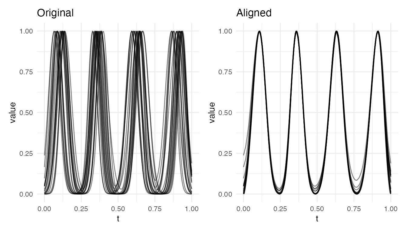
plot(res7, type = "both")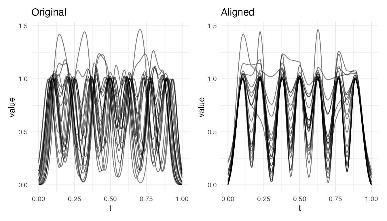
With 4 bumps, alignment still captures most of the variability. With 7 tightly packed bumps, the monotonicity constraint on the warping function limits independent correction of each peak – stretching one inter-peak region forces compression elsewhere. This is a fundamental limitation of elastic alignment, not a numerical issue: a single monotone time-warping cannot independently retime many closely spaced features.
Comparison with DTW and Shift Registration
Three alignment strategies are available in fdars:
| Elastic (SRSF) | DTW | Shift Registration | |
|---|---|---|---|
| Function | elastic.align() |
metric.DTW() |
register.fd() |
| Warping | Smooth, monotone diffeomorphism | Piecewise constant, allows repeated indices | Global translation only |
| Metric | Proper metric (triangle inequality holds) | Not a metric | Not applicable (no warping) |
| Amplitude/Phase | Cleanly separates the two | Mixes them — can absorb amplitude differences into warping | Pure phase (shift), amplitude untouched |
| Degeneracy | No “pinching” — SRSF penalizes compression | Can collapse entire regions to a single point | No degeneracy, but very limited |
| Mean | Karcher mean is well-defined | No principled mean | Shift-corrected cross-sectional mean |
| Complexity | per pair (DP) | per pair (DP) | per curve (cross-correlation) |
Why Elastic Alignment Avoids Degeneracy
A key advantage of the SRSF framework is that the elastic distance penalizes “pinching” — collapsing a region of the curve to a single point. The SRSF of a warped function is , so when (extreme compression), the SRSF contribution vanishes rather than concentrating. This acts as a natural regularizer. In contrast, DTW allows repeated indices that effectively collapse entire regions to a single point, which can produce degenerate alignments.
Head-to-Head: Shifted Bumps
The clearest way to see the differences is on data with localized features:
set.seed(42)
m_cmp <- 200
argvals_cmp <- seq(0, 1, length.out = m_cmp)
n_cmp <- 15

# Two bumps with varying positions
data_cmp <- matrix(0, n_cmp, m_cmp)
for (i in 1:n_cmp) {
  p1 <- 0.3 + runif(1, -0.06, 0.06)
  p2 <- 0.7 + runif(1, -0.06, 0.06)
  data_cmp[i, ] <- exp(-300 * (argvals_cmp - p1)^2) +
                   exp(-300 * (argvals_cmp - p2)^2)
}
fd_cmp <- fdata(data_cmp, argvals = argvals_cmp)
var_orig_cmp <- mean(apply(fd_cmp$data, 2, var))
Elastic alignment finds smooth, local warping for each bump independently:
res_elastic <- elastic.align(fd_cmp)
vr_elastic <- 1 - mean(apply(res_elastic$aligned$data, 2, var)) / var_orig_cmp
cat("Elastic VR:", round(vr_elastic * 100, 1), "%\n")
#> Elastic VR: 100 %
Shift registration applies a single global shift – it can center one bump but not both when they move independently:
res_shift <- register.fd(fd_cmp)
vr_shift <- 1 - mean(apply(res_shift$registered$data, 2, var)) / var_orig_cmp
cat("Shift registration VR:", round(vr_shift * 100, 1), "%\n")
#> Shift registration VR: -55.1 %
plot_curves <- function(data, argvals, title) {
  n <- nrow(data)
  m <- length(argvals)
  df <- data.frame(
    curve_id = rep(seq_len(n), each = m),
    argval = rep(argvals, n),
    value = as.vector(t(data))
  )
  ggplot(df, aes(x = argval, y = value, group = curve_id)) +
    geom_line(alpha = 0.5) +
    labs(title = title, x = "t", y = "value") +
    theme_minimal()
}

p1 <- plot_curves(fd_cmp$data, argvals_cmp, "Original")
p2 <- plot_curves(res_elastic$aligned$data, argvals_cmp,
        paste0("Elastic (VR = ", round(vr_elastic * 100, 1), "%)"))
p3 <- plot_curves(res_shift$registered$data, argvals_cmp,
        paste0("Shift Registration (VR = ", round(vr_shift * 100, 1), "%)"))

p1 / p2 / p3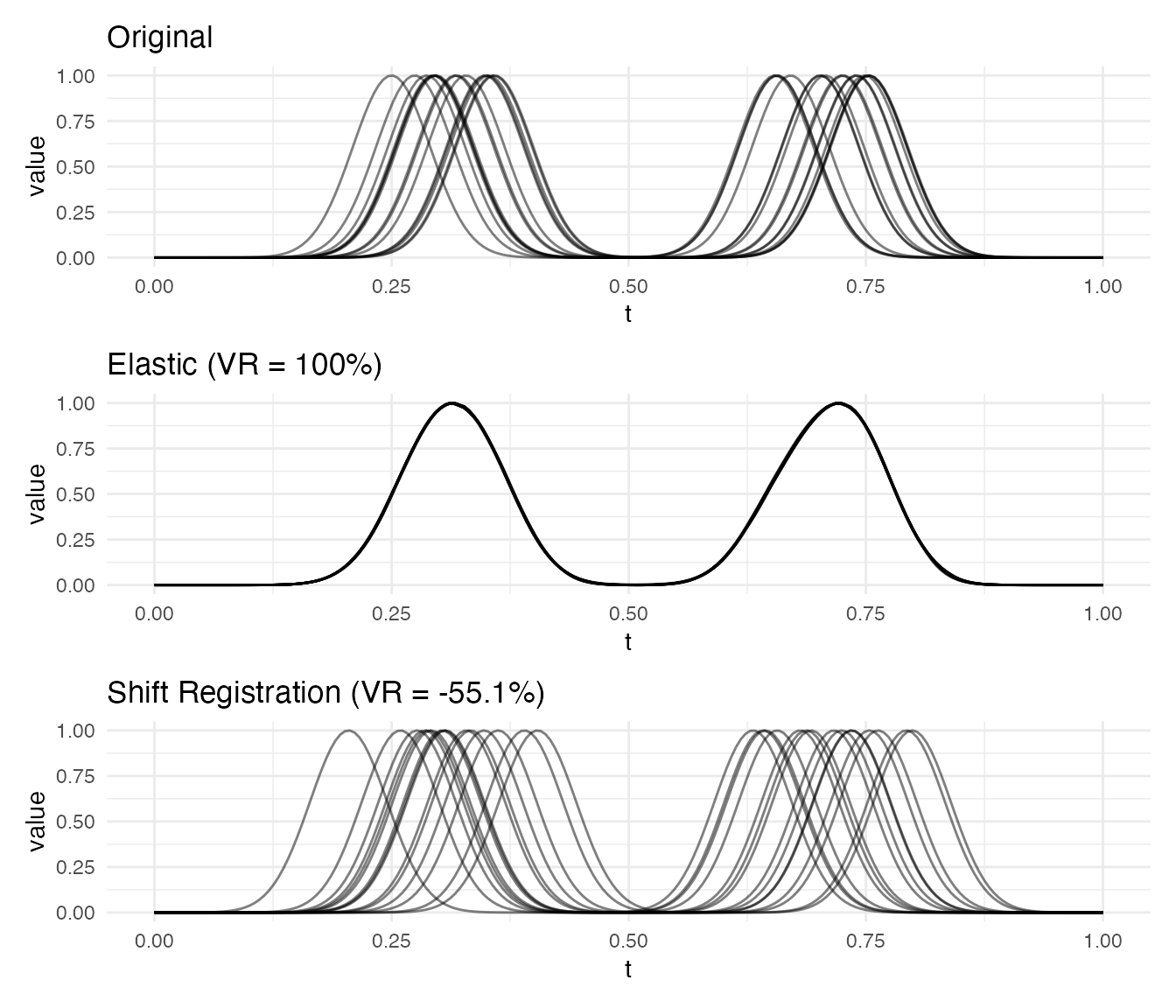
Elastic alignment resolves the independent shifts of both bumps. Shift registration can only correct a single global offset, leaving residual phase variability when features move independently.
DTW Distance vs Elastic Distance
DTW and elastic distances rank curves differently because DTW can absorb amplitude differences into warping while elastic alignment separates them:
# Compute both distance matrices
D_elastic <- elastic.distance(fd_cmp)
D_dtw <- metric.DTW(fd_cmp)

# Compare: correlation of off-diagonal entries
idx <- upper.tri(D_elastic)
cat("Correlation between elastic and DTW distances:",
    round(cor(D_elastic[idx], D_dtw[idx]), 3), "\n")
#> Correlation between elastic and DTW distances: 0.895
df_ed <- data.frame(elastic = D_elastic[idx], dtw = D_dtw[idx])
ggplot(df_ed, aes(x = elastic, y = dtw)) +
  geom_point(color = "steelblue", size = 1, alpha = 0.7) +
  geom_smooth(method = "lm", se = FALSE, color = "red", linewidth = 1.5) +
  labs(title = "Elastic vs DTW Pairwise Distances",
       x = "Elastic distance", y = "DTW distance") +
  theme_minimal()
#> `geom_smooth()` using formula = 'y ~ x'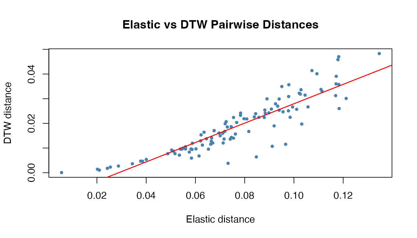
The distances are correlated but not identical. The key difference emerges when amplitude variability is present:
set.seed(42)
# Curves with BOTH amplitude and phase variability
data_amp <- matrix(0, n_cmp, m_cmp)
for (i in 1:n_cmp) {
  amp <- runif(1, 0.5, 1.5)
  shift <- runif(1, -0.06, 0.06)
  data_amp[i, ] <- amp * exp(-200 * (argvals_cmp - 0.5 - shift)^2)
}
fd_amp <- fdata(data_amp, argvals = argvals_cmp)

D_elastic_amp <- elastic.distance(fd_amp)
D_dtw_amp <- metric.DTW(fd_amp)
idx_amp <- upper.tri(D_elastic_amp)

cat("Correlation (amplitude+phase):",
    round(cor(D_elastic_amp[idx_amp], D_dtw_amp[idx_amp]), 3), "\n")
#> Correlation (amplitude+phase): 0.929
With mixed amplitude and phase, DTW distances are less correlated with elastic distances because DTW warping partially absorbs amplitude differences. Elastic distances preserve the amplitude/phase separation, making them more suitable for downstream analysis (clustering, MDS) when both sources of variability carry distinct meaning.
When to Use Each Method
| Scenario | Recommended |
|---|---|
| Localized features with independent timing shifts | Elastic alignment |
| Simple global time shift or delay | Shift registration (register.fd) — fast
and sufficient |
| Distance computation for clustering/MDS | Elastic distance (proper metric) or DTW (if metric property not needed) |
| Noisy signals, speech-like data | DTW (more robust to noise without pre-smoothing) |
| Periodic/circular data | elastic.align(periodic = TRUE) |
| Need principled mean shape |
karcher.mean() (no DTW equivalent) |
Periodic Functional Data
The Problem
Elastic alignment uses fixed boundary constraints , . This prevents the warping function from performing circular shifts, which means periodic data (e.g., curves on where ) with large phase offsets cannot be properly aligned.
For example, two copies of shifted by half a period have identical shape but the boundary constraints force alignment to fail:
set.seed(42)
m <- 100
argvals_p <- seq(0, 2 * pi, length.out = m)
n <- 15
data_p <- matrix(0, n, m)
for (i in 1:n) {
  shift <- sample(0:(m - 1), 1)
  idx <- ((seq_len(m) - 1L + shift) %% m) + 1L
  data_p[i, ] <- sin(argvals_p[idx])
}
fd_p <- fdata(data_p, argvals = argvals_p)

# Standard alignment struggles with circular shifts
res_std <- elastic.align(fd_p)
var_orig <- mean(apply(fd_p$data, 2, var))
vr_std <- 1 - mean(apply(res_std$aligned$data, 2, var)) / var_orig
cat("Standard alignment on periodic data — VR:", round(vr_std * 100, 1), "%\n")
#> Standard alignment on periodic data — VR: 66.6 %
plot(res_std, type = "both")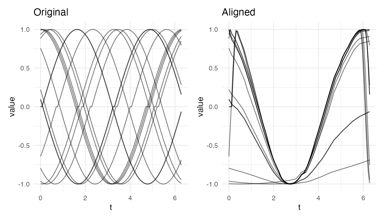
The Solution
Setting periodic = TRUE applies a two-stage
approach:
-
Circular rotation: For each curve, find the
position of the global maximum. Circularly shift the curve so that this
maximum lands at a fixed canonical grid position (by default, one
quarter of the domain). The shift for curve
is simply
which.max(f_i) - target_pos. This is a deterministic, fast heuristic – no optimisation is involved. - Elastic alignment: Standard boundary-constrained alignment on the rotated data, correcting any remaining timing differences.
Caveat: The rotation heuristic relies on a single
dominant peak. If curves have multiple peaks of similar height,
which.max may select different peaks for different curves,
producing inconsistent rotations. In such cases, you may need to supply
a custom target.pos to periodic.rotate(), or
pre-process the data to ensure a consistent landmark is the global
maximum.
res_per <- elastic.align(fd_p, periodic = TRUE)
vr_per <- 1 - mean(apply(res_per$aligned$data, 2, var)) / var_orig
cat("Periodic alignment — VR:", round(vr_per * 100, 1), "%\n")
#> Periodic alignment — VR: 100 %
plot(res_per, type = "both")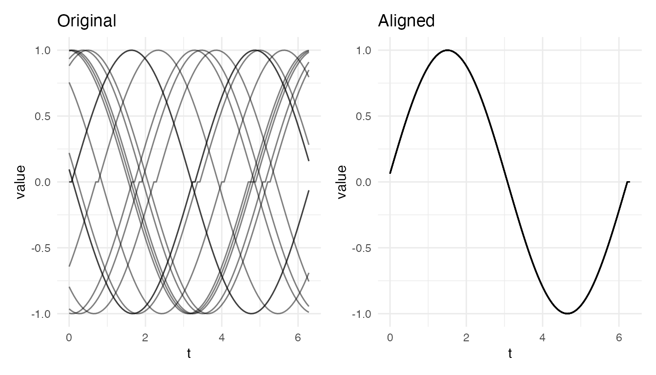
The rotation step removes large circular shifts that the boundary-constrained warping cannot handle, and the elastic step corrects any remaining timing differences.
What Happens to the Warping Functions?
Comparing the warping functions from standard vs periodic alignment reveals why the standard approach fails. Let’s look at the warping functions side by side, and inspect the warping speed:
p_warp_std <- plot(res_std, type = "warps") +
  labs(title = "Standard: warping functions")
p_warp_per <- plot(res_per, type = "warps") +
  labs(title = "Periodic: warping functions")
p_warp_std + p_warp_per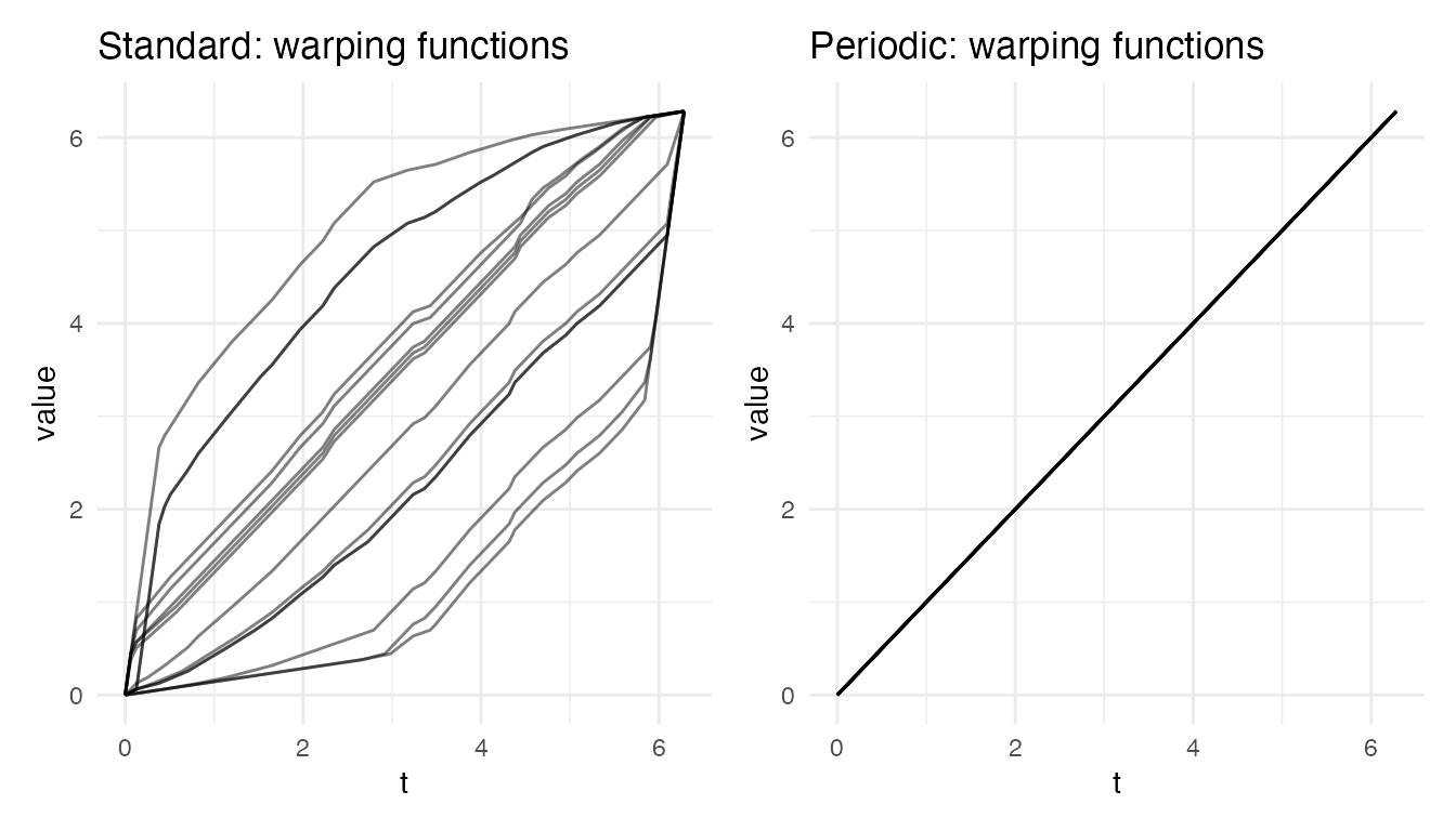
The standard warps are forced through and . When the true offset is a large circular shift, the warp must bend drastically to compensate, producing extreme stretching in some regions and compression in others. The periodic warps are much closer to the identity because the circular rotation has already removed most of the phase offset.
We can quantify this by looking at the warping speed
via deriv():
speed_std <- deriv(res_std$gammas)
speed_per <- deriv(res_per$gammas)

cat("Standard alignment — warping speed range:",
    round(min(speed_std$data), 2), "to", round(max(speed_std$data), 2), "\n")
#> Standard alignment — warping speed range: 0.14 to 7
cat("Periodic alignment — warping speed range:",
    round(min(speed_per$data), 2), "to", round(max(speed_per$data), 2), "\n")
#> Periodic alignment — warping speed range: 1 to 1
n_std <- nrow(speed_std$data)
m_std <- ncol(speed_std$data)
df_speed_std <- data.frame(
  t = rep(speed_std$argvals, n_std),
  speed = as.vector(t(speed_std$data)),
  curve = rep(seq_len(n_std), each = m_std)
)
n_per <- nrow(speed_per$data)
m_per <- ncol(speed_per$data)
df_speed_per <- data.frame(
  t = rep(speed_per$argvals, n_per),
  speed = as.vector(t(speed_per$data)),
  curve = rep(seq_len(n_per), each = m_per)
)

p_sp_std <- ggplot(df_speed_std, aes(x = t, y = speed, group = curve)) +
  geom_hline(yintercept = 1, linetype = "dashed", color = "grey60") +
  geom_line(alpha = 0.3, color = "coral") +
  labs(title = "Standard: warping speed", x = "t",
       y = expression(dot(gamma)(t)))

p_sp_per <- ggplot(df_speed_per, aes(x = t, y = speed, group = curve)) +
  geom_hline(yintercept = 1, linetype = "dashed", color = "grey60") +
  geom_line(alpha = 0.3, color = "steelblue") +
  coord_cartesian(ylim = range(df_speed_std$speed)) +
  labs(title = "Periodic: warping speed", x = "t",
       y = expression(dot(gamma)(t)))

p_sp_std + p_sp_per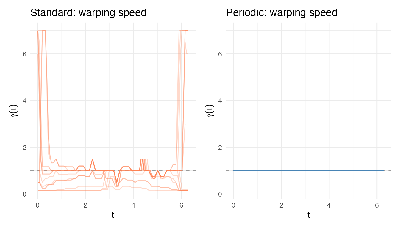
The standard warping speeds swing wildly (extreme stretching and compression), while the periodic warping speeds stay close to 1 (the identity). This illustrates the benefit of the two-stage periodic approach: the rotation handles the gross circular shift, leaving only minor residual timing differences for the elastic alignment to correct.
Let’s examine one curve in detail to see the full decomposition – the circular rotation followed by the residual elastic warp:
# Pick the curve with the largest rotation shift
rot <- periodic.rotate(fd_p)
i_max <- which.max(abs(rot$shifts))
shift_amount <- rot$shifts[i_max]

# Three stages: original, after rotation, after alignment
f_orig <- as.numeric(fd_p$data[i_max, ])
f_rotated <- as.numeric(rot$fdataobj$data[i_max, ])
f_aligned <- as.numeric(res_per$aligned$data[i_max, ])
f_target <- as.numeric(res_per$target)

# Panel 1: the three curve stages
df_stages <- data.frame(
  t = rep(argvals_p, 4),
  value = c(f_orig, f_rotated, f_aligned, f_target),
  stage = rep(c("1. Original", "2. After rotation", "3. After alignment",
                "Target"), each = m)
)

p1 <- ggplot(df_stages, aes(x = t, y = value, color = stage,
                             linetype = stage)) +
  geom_line(linewidth = 0.9) +
  scale_color_manual(values = c("1. Original" = "coral",
                                "2. After rotation" = "goldenrod",
                                "3. After alignment" = "steelblue",
                                "Target" = "grey30")) +
  scale_linetype_manual(values = c("1. Original" = "solid",
                                   "2. After rotation" = "solid",
                                   "3. After alignment" = "solid",
                                   "Target" = "dashed")) +
  labs(title = paste0("Curve ", i_max, ": two-stage periodic alignment",
                      " (rotation = ", shift_amount, " grid points)"),
       x = "t", y = "value", color = NULL, linetype = NULL) +
  theme(legend.position = "top")

# Panel 2: warping function (standard vs periodic)
gamma_std <- as.numeric(res_std$gammas$data[i_max, ])
gamma_per <- as.numeric(res_per$gammas$data[i_max, ])
df_warps <- data.frame(
  t = rep(argvals_p, 2),
  gamma = c(gamma_std, gamma_per),
  method = rep(c("Standard", "Periodic"), each = m)
)

p2 <- ggplot(df_warps, aes(x = t, y = gamma, color = method)) +
  geom_abline(slope = 1, intercept = 0, linetype = "dashed", color = "grey60") +
  geom_line(linewidth = 1) +
  scale_color_manual(values = c(Standard = "coral", Periodic = "steelblue")) +
  labs(title = "Warping function: standard vs periodic",
       x = "t", y = expression(gamma(t)), color = NULL) +
  theme(legend.position = "top")

# Panel 3: warping speed comparison
speed_std_i <- as.numeric(deriv(res_std$gammas)$data[i_max, ])
speed_per_i <- as.numeric(deriv(res_per$gammas)$data[i_max, ])
df_sp <- data.frame(
  t = rep(deriv(res_per$gammas)$argvals, 2),
  speed = c(speed_std_i, speed_per_i),
  method = rep(c("Standard", "Periodic"), each = length(speed_per_i))
)

p3 <- ggplot(df_sp, aes(x = t, y = speed, color = method)) +
  geom_hline(yintercept = 1, linetype = "dashed", color = "grey60") +
  geom_line(linewidth = 0.8) +
  scale_color_manual(values = c(Standard = "coral", Periodic = "steelblue")) +
  labs(title = "Local warping speed: deriv(gammas)",
       x = "t", y = expression(dot(gamma)(t)), color = NULL) +
  theme(legend.position = "top")

p1 / p2 / p3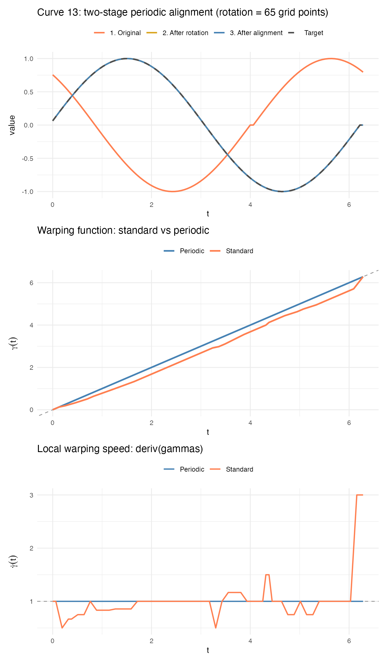
The three panels show the full story for this curve:
- Top: The original curve (coral) is circularly shifted far from the target. Rotation (gold) brings it close; the residual elastic warp (blue) finishes the job.
- Middle: The standard warping function (coral) deviates wildly from the diagonal because it must encode a large circular shift as a boundary- constrained warp. The periodic warping function (blue) stays near the identity.
- Bottom: The standard warp speed swings between extreme compression and stretching. The periodic warp speed is nearly constant at 1.
Where Did the Shift Go?
Notice that the periodic warping function is nearly the identity – it
does not show the large circular shift visible in the
original data. This is because the shift was already removed by
periodic.rotate() before the elastic alignment
runs. The total phase correction in the periodic approach is decomposed
into two pieces:
-
Circular rotation (stored in
res_per$rotations) – the gross shift, measured in grid points -
Elastic warp (stored in
res_per$gammas) – the residual fine-tuning
You can inspect both:
cat("Curve", i_max, "phase decomposition:\n")
#> Curve 13 phase decomposition:
cat("  Circular rotation:", res_per$rotations[i_max], "grid points (",
    round(res_per$rotations[i_max] / m * 2 * pi, 2), "radians)\n")
#>   Circular rotation: 65 grid points ( 4.08 radians)
warp_deviation <- as.numeric(res_per$gammas$data[i_max, ]) - argvals_p
cat("  Residual warp: mean |gamma(t) - t| =",
    round(mean(abs(warp_deviation)), 4), "\n")
#>   Residual warp: mean |gamma(t) - t| = 0
This decomposition is the key difference from the non-periodic case. In the Quick Start example, the warping function had to absorb the entire shift, producing a visible deviation from the diagonal. Here, the rotation absorbs the gross shift, and the warping function only encodes what’s left.
Alternative Rotation Methods
The default "peak" rotation uses which.max
to locate each curve’s global maximum and shift it to a canonical
position. This is fast but fragile when curves have multiple
peaks of similar height – which.max may pick
different peaks for different curves, producing inconsistent
rotations.
Three additional methods are available via the method
argument to periodic.rotate() (and via
rotate.method in elastic.align() and
karcher.mean()):
Cross-correlation (method = "xcorr")
Cross-correlation finds the circular shift that best aligns each curve to a reference, using all features simultaneously rather than a single landmark. This is robust to multi-peak shapes:
# Multi-peak curves where peak method fails
set.seed(42)
base_multi <- sin(argvals_p) + 0.95 * sin(2 * argvals_p + 0.3)
n_multi <- 12
data_multi <- matrix(0, n_multi, m)
for (i in 1:n_multi) {
  shift <- sample(0:(m - 1), 1)
  idx <- ((seq_len(m) - 1L + shift) %% m) + 1L
  data_multi[i, ] <- base_multi[idx]
}
fd_multi <- fdata(data_multi, argvals = argvals_p)

rot_peak <- periodic.rotate(fd_multi, method = "peak")
rot_xcorr <- periodic.rotate(fd_multi, method = "xcorr")

# Compare variance reduction
var_orig <- mean(apply(fd_multi$data, 2, var))
vr_peak <- 1 - mean(apply(rot_peak$fdataobj$data, 2, var)) / var_orig
vr_xcorr <- 1 - mean(apply(rot_xcorr$fdataobj$data, 2, var)) / var_orig
cat("Multi-peak rotation VR — peak:", round(vr_peak * 100, 1), "%,",
    "xcorr:", round(vr_xcorr * 100, 1), "%\n")
#> Multi-peak rotation VR — peak: 100 %, xcorr: 100 %
p_peak <- plot(rot_peak$fdataobj) + labs(title = "Peak rotation")
p_xcorr <- plot(rot_xcorr$fdataobj) + labs(title = "Cross-correlation rotation")
p_peak + p_xcorr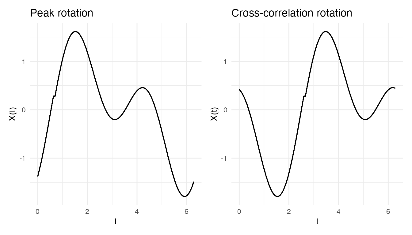
The cross-correlation method aligns curves coherently because it
matches the entire shape rather than a single point.
You can supply a custom reference via the reference
argument; by default it uses the cross-sectional mean.
Landmark-based (method = "landmark")
The landmark method generalises the peak approach: instead of
which.max, you supply any function that locates a feature
of interest. For example, a “steepest rise” function finds the point of
maximum first derivative:
steepest_rise <- function(curve) {
  diffs <- diff(curve)
  which.max(diffs)
}

rot_lm <- periodic.rotate(fd_p, method = "landmark",
                           landmark.func = steepest_rise)
cat("Landmark shifts:", rot_lm$shifts, "\n")
#> Landmark shifts: 28 12 52 3 -23 59 28 30 53 6 -23 -12 40 57 51
This is useful when the relevant feature isn’t the peak but some other characteristic point – a zero crossing, the start of a rise, etc.
Iterative (method = "iterative")
The iterative method alternates between cross-correlation rotation and elastic alignment. This handles cases where the optimal rotation depends on the alignment and vice versa:
rot_iter <- periodic.rotate(fd_p, method = "iterative", max.iter = 5)
cat("Iterative shifts:", rot_iter$shifts, "\n")
#> Iterative shifts: 82 66 6 57 31 13 82 84 7 60 31 42 94 11 5
The iterative approach converges when no further shifts are needed (all lags become zero). It is the most expensive method but can improve results when curves have complex shapes.
When to Use Each Method
| Method | Best for | Cost |
|---|---|---|
"peak" |
Single dominant peak, fast pre-screening | O(m) per curve |
"xcorr" |
Multi-peak curves, noisy data | O(m log m) per curve |
"landmark" |
Domain-specific features (zero crossing, onset) | O(m) per curve |
"iterative" |
Complex shapes where rotation and alignment interact | O(m log m) × iters |
You can pass the rotation method through to
elastic.align() and karcher.mean() via the
rotate.method parameter:
res_xcorr <- elastic.align(fd_multi, periodic = TRUE, rotate.method = "xcorr")
print(res_xcorr)
#> Elastic Alignment
#>   Curves: 12 x 100 grid points
#>   Mean elastic distance: 0
#>   Periodic: TRUE (method: xcorr )
You can also apply the rotation step manually using
periodic.rotate():
rot <- periodic.rotate(fd_p)
cat("Shifts applied:", rot$shifts, "\n")
#> Shifts applied: 53 37 -23 28 2 -16 53 55 -22 31 2 13 65 -18 -24
The karcher.mean() function also accepts
periodic = TRUE:
km_per <- karcher.mean(fd_p, max.iter = 15, periodic = TRUE)
print(km_per)
#> Karcher Mean (Elastic)
#>   Curves: 15 x 100 grid points
#>   Iterations: 10
#>   Converged: FALSE
#>   Periodic: TRUE (method: peak )
Real Data: Berkeley Growth Velocity
For a full worked example applying elastic alignment, Karcher mean,
FPCA, and equivalence testing to the Berkeley Growth Study data, see
vignette("articles/example-berkeley-growth").
Practical Tips
Pre-smooth Noisy Data
The SRSF transform involves derivatives, so noise gets amplified. Always smooth noisy data before alignment:
set.seed(42)
noisy <- matrix(0, 15, 100)
shifts <- runif(15, -0.1, 0.1)
for (i in 1:15) {
  noisy[i, ] <- sin(2 * pi * (argvals - shifts[i])) + rnorm(100, sd = 0.15)
}
fd_noisy <- fdata(noisy, argvals = argvals)

# Smooth with B-spline basis
coefs <- fdata2basis(fd_noisy, nbasis = 15, type = "bspline")
fd_smooth <- basis2fdata(coefs, argvals)

var_before <- mean(apply(fd_noisy$data, 2, var))

# Align raw vs smoothed
res_raw <- elastic.align(fd_noisy)
res_smooth <- elastic.align(fd_smooth)

vr_raw <- 1 - mean(apply(res_raw$aligned$data, 2, var)) / var_before
vr_smooth <- 1 - mean(apply(res_smooth$aligned$data, 2, var)) / var_before
cat("VR (raw):     ", round(vr_raw * 100, 1), "%\n")
#> VR (raw):      47.5 %
cat("VR (smoothed):", round(vr_smooth * 100, 1), "%\n")
#> VR (smoothed): 81.7 %
Use Sufficient Grid Resolution
The dynamic programming alignment operates on the evaluation grid. Finer grids yield more accurate warping:
set.seed(42)
for (m in c(20, 50, 100, 200)) {
  av <- seq(0, 1, length.out = m)
  shifts <- runif(15, -0.1, 0.1)
  dm <- matrix(0, 15, m)
  for (i in 1:15) dm[i, ] <- sin(2 * pi * (av - shifts[i]))
  fd_m <- fdata(dm, argvals = av)
  ea <- elastic.align(fd_m)
  var_red <- 1 - mean(apply(ea$aligned$data, 2, var)) /
                  mean(apply(fd_m$data, 2, var))
  cat(sprintf("  m = %3d: VR = %5.1f%%\n", m, var_red * 100))
}
#>   m =  20: VR =  62.7%
#>   m =  50: VR =  73.9%
#>   m = 100: VR =  76.4%
#>   m = 200: VR =  77.2%
A minimum of 50-100 grid points is recommended.
Choose an Appropriate Target
The target curve affects alignment quality. Three options:
| Target | When to use |
|---|---|
| Cross-sectional mean (default) | General-purpose; robust with many curves |
| Deepest curve | When outliers may distort the mean |
| Known reference | When aligning to a standard template |
set.seed(42)
shifts <- runif(15, -0.1, 0.1)
dm <- matrix(0, 15, 100)
for (i in 1:15) dm[i, ] <- sin(2 * pi * (argvals - shifts[i]))
fd <- fdata(dm, argvals = argvals)
var_before <- mean(apply(fd$data, 2, var))

# Default (cross-sectional mean)
vr1 <- 1 - mean(apply(elastic.align(fd)$aligned$data, 2, var)) / var_before

# Deepest curve
depths <- depth(fd, method = "FM")
vr2 <- 1 - mean(apply(elastic.align(fd, target = fd[which.max(depths)])$aligned$data, 2, var)) / var_before

cat("Cross-sectional mean: VR =", round(vr1 * 100, 1), "%\n")
#> Cross-sectional mean: VR = 75.9 %
cat("Deepest curve:        VR =", round(vr2 * 100, 1), "%\n")
#> Deepest curve:        VR = 75.7 %
Alignment + FPCA
Alignment before FPCA concentrates variance into the first principal component by removing phase variability that would otherwise spread across components:
set.seed(42)
shifts <- runif(15, -0.1, 0.1)
dm <- matrix(0, 15, 100)
for (i in 1:15) dm[i, ] <- sin(2 * pi * (argvals - shifts[i]))
fd <- fdata(dm, argvals = argvals)

# FPCA before and after alignment
pc_before <- fdata2pc(fd, ncomp = 3)
ea <- elastic.align(fd)
pc_after <- fdata2pc(ea$aligned, ncomp = 3)

pve_before <- round(pc_before$d^2 / sum(pc_before$d^2) * 100, 1)
pve_after <- round(pc_after$d^2 / sum(pc_after$d^2) * 100, 1)

cat("Before alignment: PC1 =", pve_before[1], "%, PC2 =", pve_before[2], "%\n")
#> Before alignment: PC1 = 97.8 %, PC2 = 2.2 %
cat("After alignment:  PC1 =", pve_after[1], "%, PC2 =", pve_after[2], "%\n")
#> After alignment:  PC1 = 99.1 %, PC2 = 0.7 %
Limitations
Fixed Boundary Conditions
Warping functions are constrained to and . This means the alignment cannot correct mismatches at the domain boundaries. For shifted curves, the residual at the boundary equals the value difference:
f1 <- sin(2 * pi * argvals)
f2 <- sin(2 * pi * (argvals - 0.1))

fd2 <- fdata(rbind(f1, f2), argvals = argvals)
ea <- elastic.align(fd2)

# Boundary residual = |sin(0) - sin(-0.2*pi)| = 0.588
cat("Boundary gap:          ", round(abs(f2[1] - f1[1]), 3), "\n")
#> Boundary gap:           0.588
cat("Max aligned difference:", round(max(abs(ea$aligned$data[1, ] - ea$aligned$data[2, ])), 3), "\n")
#> Max aligned difference: 0.588
cat("Interior max diff:     ", round(max(abs(ea$aligned$data[1, 10:90] - ea$aligned$data[2, 10:90])), 3), "\n")
#> Interior max diff:      0.339
The interior alignment is excellent even when boundaries cannot be corrected.
Amplitude-Only Differences
When curves differ only in amplitude (e.g., vs ), alignment correctly produces identity warping – no spurious time distortion:
f1 <- sin(2 * pi * argvals)
f2 <- 2 * sin(2 * pi * argvals)
fd_amp <- fdata(rbind(f1, f2), argvals = argvals)
res_amp <- elastic.align(fd_amp)

max_warp_dev <- max(abs(res_amp$gammas$data -
                        matrix(argvals, 2, 100, byrow = TRUE)))
cat("Max warp deviation from identity:", max_warp_dev, "\n")
#> Max warp deviation from identity: 0
This is the correct behavior: amplitude differences should not produce warping. However, when both amplitude and phase variability are present, the phase correction may be partial – alignment focuses on phase and leaves amplitude untouched.
Domain Independence
The alignment works correctly on any domain, not just :
for (domain in list(c(0, 1), c(0, 2*pi), c(0, 10), c(-1, 1))) {
  av <- seq(domain[1], domain[2], length.out = 100)
  range <- domain[2] - domain[1]
  dm <- matrix(0, 10, 100)
  set.seed(42)
  for (i in 1:10) {
    shift <- runif(1, -0.1 * range, 0.1 * range)
    dm[i, ] <- sin(2 * pi * (av - shift) / range)
  }
  fd <- fdata(dm, argvals = av)
  ea <- elastic.align(fd)
  var_red <- 1 - mean(apply(ea$aligned$data, 2, var)) /
                 mean(apply(fd$data, 2, var))
  cat(sprintf("  [%g, %g]: VR = %.1f%%\n", domain[1], domain[2], var_red * 100))
}
#>   [0, 1]: VR = 76.1%
#>   [0, 6.28319]: VR = 76.1%
#>   [0, 10]: VR = 76.1%
#>   [-1, 1]: VR = 76.1%
Lambda Selection via Cross-Validation
The regularization parameter lambda controls the
trade-off between alignment quality and warp smoothness. Use
elastic.lambda.cv() to select it automatically via K-fold
cross-validation:
set.seed(42)
n <- 30; m <- 50
av <- seq(0, 1, length.out = m)
X <- matrix(0, n, m)
for (i in 1:n) {
  shift <- runif(1, -0.1, 0.1)
  X[i, ] <- sin(2 * pi * (av + shift)) + rnorm(m, sd = 0.1)
}
fd_cv <- fdata(X, argvals = av)

cv_result <- elastic.lambda.cv(fd_cv,
                                lambdas = 10^seq(-3, 1, length.out = 10),
                                n.folds = 5, seed = 42)
cv_result
#> Lambda Cross-Validation
#>   Candidates tested: 10
#>   Best lambda: 0.007743
#>   Best CV score: 1.098
plot(cv_result)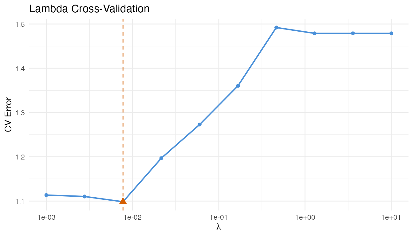
The optimal lambda minimizes the CV reconstruction error.
Warp Statistics
After computing a Karcher mean, examine the warping functions with
warp.statistics(). This provides pointwise mean, standard
deviation, and confidence bands:
km <- karcher.mean(fd_cv, max.iter = 15)
ws <- warp.statistics(km)
ws
#> Warping Function Statistics
#>   Grid points: 50
#>   Curves: 30
#>   Mean geodesic distance: 0.2698
#>   Max geodesic distance: 0.3903
plot(ws)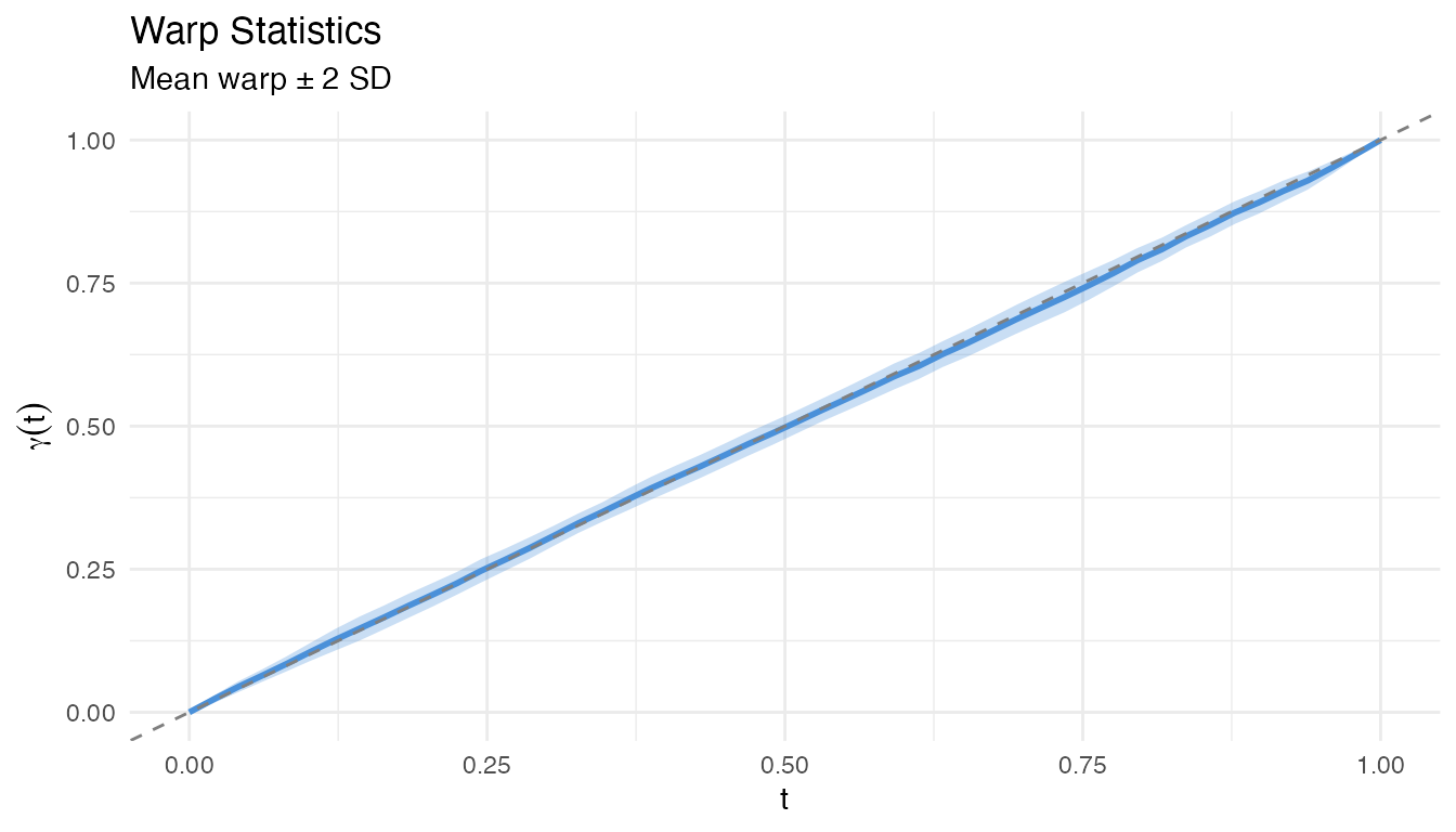
The plot shows the mean warp (solid) with a 95% confidence band (shaded). Warps far from the identity indicate strong phase variation at those domain locations.
Phase Boxplots
Phase boxplots provide a functional boxplot of the warping functions, identifying outlier warps:
pb <- phase.boxplot(km, factor = 1.5)
pb
#> Phase Boxplot (Warping Functions)
#>   Grid points: 50
#>   Curves: 30
#>   Median index: 11
#>   Outliers: 0
#>   Factor: 1.5
plot(pb)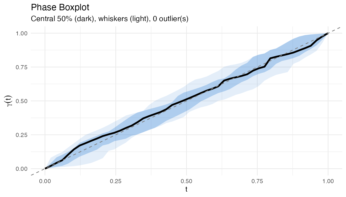
The central 50% region (darker shading) contains the typical warps, while curves outside the whiskers are flagged as phase outliers.
Registration Diagnostics
alignment.diagnostics() assesses per-curve alignment
quality, detecting under-alignment, over-alignment, and non-monotone
warps:
diag <- alignment.diagnostics(fd_cv, km)
diag
#> Alignment Diagnostics
#>   Curves: 30
#>   Flagged: 30 of 30 (100%)
#>   Health score: 0
#>   Flagged indices: 1, 2, 3, 4, 5, 6, 7, 8, 9, 10, 11, 12, 13, 14, 15, 16, 17, 18, 19, 20, 21, 22, 23, 24, 25, 26, 27, 28, 29, 30
plot(diag)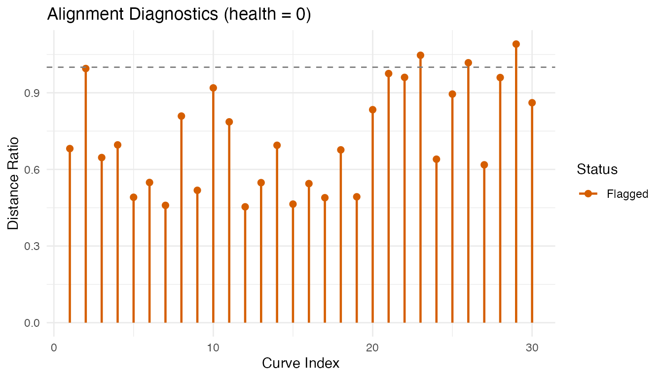
The health score (fraction of non-flagged curves) provides a quick summary. Flagged curves may need manual inspection or different alignment parameters.
For pairwise diagnostics, use
alignment.diagnostics.pairwise() to check a single pair
alignment:
f1 <- fdata(matrix(fd_cv$data[1, ], nrow = 1), argvals = av)
f2 <- fdata(matrix(fd_cv$data[2, ], nrow = 1), argvals = av)
pair <- elastic.pair(f1, f2)
diag_pair <- alignment.diagnostics.pairwise(
  fd_cv$data[1, ], fd_cv$data[2, ],
  list(gamma = pair$gamma, f.aligned = pair$f.aligned, distance = pair$distance),
  av
)
cat("Flagged:", diag_pair$flagged, "\n")
#> Flagged: TRUE
cat("Distance ratio:", round(diag_pair$distance.ratio, 3), "\n")
#> Distance ratio: 0.548
References
- Srivastava, A., Klassen, E., Joshi, S.H., and Jermyn, I.H. (2011). Shape analysis of elastic curves in Euclidean spaces. IEEE Transactions on Pattern Analysis and Machine Intelligence, 33(7):1415–1428.
- Tucker, J.D., Wu, W., and Srivastava, A. (2013). Generative models for functional data using phase and amplitude separation. Computational Statistics & Data Analysis, 61:50–66.
- Srivastava, A. and Klassen, E. (2016). Functional and Shape Data Analysis. Springer.
See Also
- Advanced Elastic Alignment – Bayesian alignment, robust Karcher mean, elastic depth, closed curves, partial matching, geodesic interpolation, and more (fdars-core 0.10.0 features)