Conformal Prediction Guide
Source:vignettes/articles/conformal-prediction-guide.Rmd
conformal-prediction-guide.RmdOverview
fdars provides 14 conformal prediction functions covering regression, classification, and elastic models. This guide helps you choose the right function for your problem and summarizes the available options.
All conformal methods share the same guarantee: for coverage level ,
holds for any data distribution, with no parametric assumptions.
Decision Flowchart

Choose your conformal method based on three questions:
1. Regression or classification?
- Regression (predict a number ) prediction intervals
- Classification (predict a label ) prediction sets
2. Which base model?
| Model | Regression | Classification |
|---|---|---|
fregre.lm |
conformal.fregre.lm() |
— |
fregre.np |
conformal.fregre.np() |
— |
| Elastic regression | conformal.elastic.regression() |
— |
| Elastic PCR | conformal.elastic.pcr() |
— |
| LDA / QDA / kNN | — | conformal.classif() |
| Logistic | conformal.logistic() |
conformal.elastic.logistic() |
3. How much data can you afford?
| Variant | Data use | # fits | Guarantee | Function suffix |
|---|---|---|---|---|
| Split | Wastes calibration fraction | 1 | model-specific | |
| CV+ | All data used | folds | cv.conformal.*() |
|
| Jackknife+ | All data used | LOO fits | jackknife.plus() |
|
| Generic | Pre-fitted model | 0 | Heuristic only | conformal.generic.*() |
Caveat: Generic conformal uses a model trained on ALL data including the calibration set, so calibration residuals are in-sample. The coverage guarantee is broken. Use split or CV+ methods for valid coverage.
Complete Function Reference
Split Conformal — Regression

Each function takes training fdata, response
y, test fdata, and returns prediction
intervals.
| Function | Model | Key parameters |
|---|---|---|
conformal.fregre.lm() |
FPC linear |
ncomp, cal.fraction
|
conformal.fregre.np() |
Nonparametric |
ncomp, cal.fraction
|
conformal.elastic.regression() |
Elastic regression |
ncomp, cal.fraction
|
conformal.elastic.pcr() |
Elastic PCR |
ncomp, cal.fraction
|
conformal.logistic() |
Logistic (binary) |
ncomp, cal.fraction
|
All return: predictions, lower,
upper, residual.quantile,
coverage.
Split Conformal — Classification

| Function | Model | Key parameters |
|---|---|---|
conformal.classif() |
LDA, QDA, kNN |
classifier, score.type
|
conformal.elastic.logistic() |
Elastic logistic |
score.type, cal.fraction
|
Returns: predicted_classes, set_sizes,
average_set_size, coverage,
score_quantile.
Cross-Conformal (CV+)

| Function | Task | Key parameters |
|---|---|---|
cv.conformal.regression() |
Regression |
method (“fregre.lm” or “fregre.np”),
n.folds
|
cv.conformal.classification() |
Classification |
classifier, score.type,
n.folds
|
Jackknife+
| Function | Task | Key parameters |
|---|---|---|
jackknife.plus() |
Regression |
method (“fregre.lm” or “fregre.np”) |
Generic Conformal (pre-fitted model)
| Function | Task | Input model |
|---|---|---|
conformal.generic.regression() |
Regression | Fitted fregre.lm object |
conformal.generic.classification() |
Classification | Fitted functional.logistic object |
Worked Example: Regression
We simulate a realistic near-infrared spectroscopy scenario: 200 absorbance curves measured at 100 wavelengths, with a scalar response (e.g., fat content) that depends on a localized spectral region. The goal is to predict the response for 40 new spectra with valid uncertainty quantification.
set.seed(42)
n <- 200
m <- 100
t_grid <- seq(0, 1, length.out = m)

# Simulate spectra with realistic structure:
# - smooth baseline (low-freq Fourier)
# - absorption peak near t = 0.4 that varies across samples
# - measurement noise
X <- matrix(0, n, m)
for (i in 1:n) {
  baseline <- 0.8 * sin(pi * t_grid) + 0.3 * cos(2 * pi * t_grid)
  peak_loc <- 0.4 + rnorm(1, sd = 0.03)
  peak_height <- rnorm(1, mean = 2, sd = 0.6)
  X[i, ] <- baseline + peak_height * dnorm(t_grid, peak_loc, 0.05) +
            rnorm(m, sd = 0.08)
}

# Response depends on the peak region (t ∈ [0.3, 0.5])
beta_true <- dnorm(t_grid, 0.4, 0.06)
beta_true <- beta_true / max(beta_true)
dt <- t_grid[2] - t_grid[1]
y <- numeric(n)
for (i in 1:n) y[i] <- sum(beta_true * X[i, ]) * dt + rnorm(1, sd = 0.15)

# 80/20 train-test split
train_idx <- 1:160
test_idx <- 161:200
fd_train <- fdata(X[train_idx, ], argvals = t_grid)
fd_test <- fdata(X[test_idx, ], argvals = t_grid)
y_train <- y[train_idx]
y_test <- y[test_idx]
df_spectra <- data.frame(
  t = rep(t_grid, 20),
  value = as.vector(t(X[1:20, ])),
  curve = factor(rep(1:20, each = m))
)

ggplot(df_spectra, aes(x = .data$t, y = .data$value,
                       group = .data$curve)) +
  geom_line(alpha = 0.4, color = "#4A90D9") +
  labs(title = "Simulated Absorbance Spectra (first 20)",
       x = "Wavelength (normalized)", y = "Absorbance")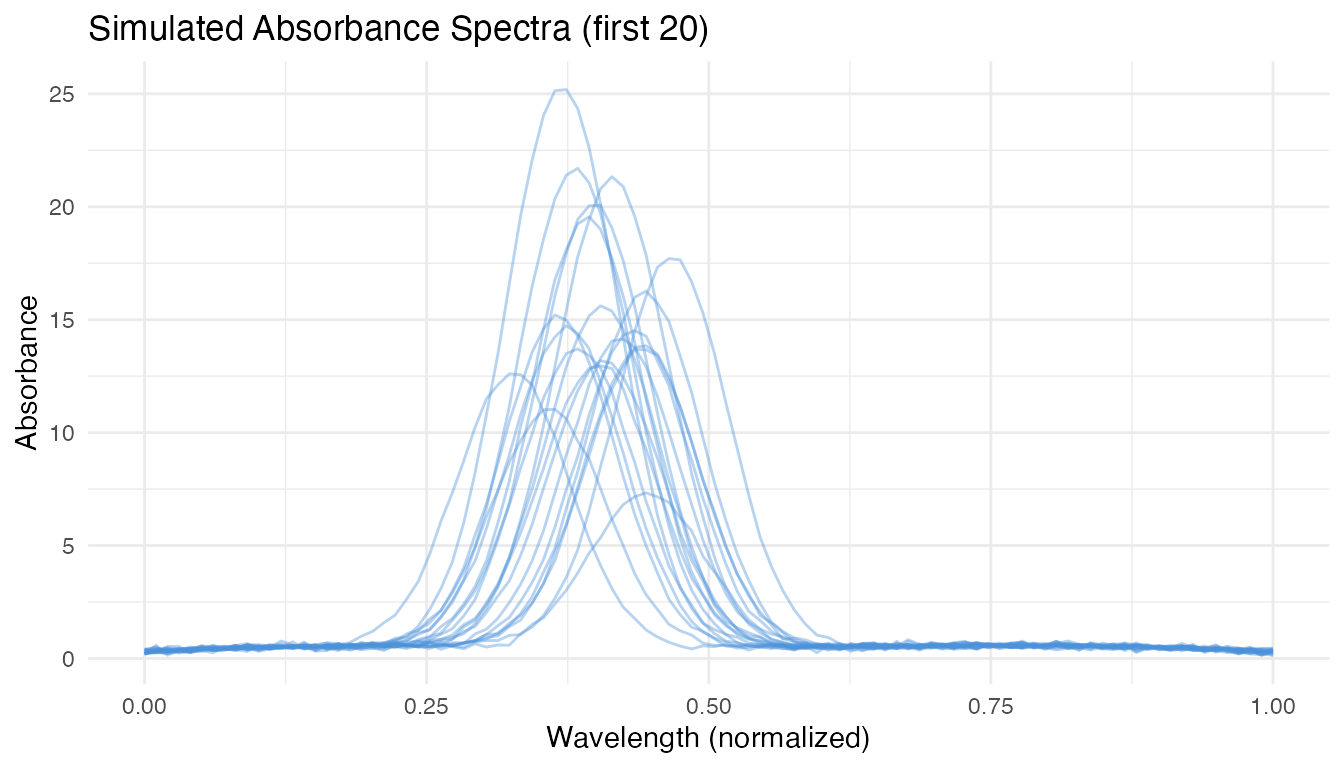
When to Use Split Conformal
Use split conformal when you have plenty of data () and want the strongest guarantee (). It only fits the model once, so it’s the fastest option. The trade-off: it “wastes” 25% of training data on calibration, producing slightly wider intervals.
split_res <- conformal.fregre.lm(
  fd_train, y_train, fd_test,
  ncomp = 5, cal.fraction = 0.25,
  alpha = 0.10, seed = 42
)

cat("Split conformal:\n")
#> Split conformal:
cat("  Coverage:", round(split_res$coverage * 100, 1), "%\n")
#>   Coverage: 92.5 %
cat("  Mean width:", round(mean(split_res$upper - split_res$lower), 4), "\n")
#>   Mean width: 0.5427
When to Use CV+
Use CV+ when data is limited () or when you want tighter intervals. All data contributes to both training and calibration through -fold cross-validation. The theoretical guarantee is weaker (), but empirically coverage is near . Cost: model fits instead of 1.
cv_res <- cv.conformal.regression(
  fd_train, y_train, fd_test,
  method = "fregre.lm", ncomp = 5,
  n.folds = 5, alpha = 0.10, seed = 42
)

cat("CV+ conformal (fregre.lm):\n")
#> CV+ conformal (fregre.lm):
cat("  Coverage:", round(cv_res$coverage * 100, 1), "%\n")
#>   Coverage: 90.6 %
cat("  Mean width:", round(mean(cv_res$upper - cv_res$lower), 4), "\n")
#>   Mean width: 0.497
CV+ also works with nonparametric models — useful when the relationship between spectra and response is nonlinear:
cv_np <- cv.conformal.regression(
  fd_train, y_train, fd_test,
  method = "fregre.np", ncomp = 5,
  n.folds = 5, alpha = 0.10, seed = 42
)

cat("CV+ conformal (fregre.np):\n")
#> CV+ conformal (fregre.np):
cat("  Coverage:", round(cv_np$coverage * 100, 1), "%\n")
#>   Coverage: 90.6 %
cat("  Mean width:", round(mean(cv_np$upper - cv_np$lower), 4), "\n")
#>   Mean width: 4.2679
When to Use Jackknife+
Use jackknife+ when you want maximum data efficiency and can afford model fits. Every observation is left out exactly once, giving the most precise calibration. Best for small-to-moderate datasets ().
jk_res <- jackknife.plus(
  fd_train, y_train, fd_test,
  method = "fregre.lm", ncomp = 5,
  alpha = 0.10
)

cat("Jackknife+:\n")
#> Jackknife+:
cat("  Coverage:", round(jk_res$coverage * 100, 1), "%\n")
#>   Coverage: 90.6 %
cat("  Mean width:", round(mean(jk_res$upper - jk_res$lower), 4), "\n")
#>   Mean width: 0.5799
When to Use Generic Conformal
Use generic conformal when the model is already fitted and you want a quick heuristic for prediction intervals without re-training.
Important: Generic conformal uses calibration residuals computed on data the model was trained on (in-sample). This means intervals are typically too narrow and the coverage guarantee
P(y in C) >= 1 - alphadoes not hold. For valid coverage, preferconformal.fregre.lm(),cv.conformal.regression(), orjackknife.plus().
model_fitted <- fregre.lm(fd_train, y_train, ncomp = 5)

gen_res <- conformal.generic.regression(
  model_fitted, fd_train, y_train, fd_test,
  cal.fraction = 0.25, alpha = 0.10, seed = 42
)
#> Warning: conformal.generic.regression uses the pre-fitted model without
#> refitting. Calibration residuals are in-sample, so coverage guarantee is
#> broken. Supply calibration.indices (held-out indices) for valid coverage, or
#> use conformal.fregre.lm() / cv.conformal.regression() instead.

cat("Generic conformal (from fitted model):\n")
#> Generic conformal (from fitted model):
cat("  Coverage:", round(gen_res$coverage * 100, 1), "%\n")
#>   Coverage: 92.5 %
cat("  Mean width:", round(mean(gen_res$upper - gen_res$lower), 4), "\n")
#>   Mean width: 0.5376
Comparing All Methods
methods <- c("Split", "CV+ (lm)", "CV+ (np)", "Jackknife+", "Generic")
widths <- list(
  split_res$upper - split_res$lower,
  cv_res$upper - cv_res$lower,
  cv_np$upper - cv_np$lower,
  jk_res$upper - jk_res$lower,
  gen_res$upper - gen_res$lower
)

df_compare <- data.frame(
  Method = rep(methods, each = length(y_test)),
  Width = unlist(widths)
)
df_compare$Method <- factor(df_compare$Method, levels = methods)

ggplot(df_compare, aes(x = .data$Method, y = .data$Width,
                       fill = .data$Method)) +
  geom_boxplot(alpha = 0.7) +
  scale_fill_manual(values = c("Split" = "#2E8B57", "CV+ (lm)" = "#4A90D9",
                                "CV+ (np)" = "#6BAED6", "Jackknife+" = "#D55E00",
                                "Generic" = "#7B2D8E")) +
  labs(title = "Prediction Interval Width by Conformal Method",
       subtitle = "All at 90% nominal level, n = 160 training curves",
       y = "Interval Width") +
  theme(legend.position = "none")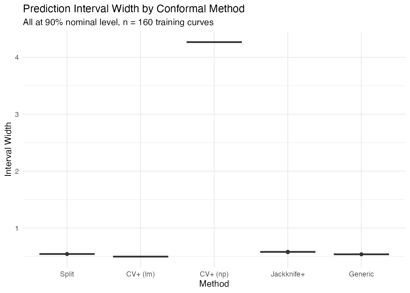
df_summary <- data.frame(
  Method = methods,
  Coverage = sapply(list(split_res, cv_res, cv_np, jk_res, gen_res),
                    function(r) round(r$coverage * 100, 1)),
  Mean_Width = sapply(widths, function(w) round(mean(w), 4)),
  Fits = c("1", "5", "5", "160", "0")
)
knitr::kable(df_summary, col.names = c("Method", "Coverage (%)",
             "Mean Width", "Model Fits"),
caption = "Conformal method comparison on spectroscopy data")| Method | Coverage (%) | Mean Width | Model Fits |
|---|---|---|---|
| Split | 92.5 | 0.5427 | 1 |
| CV+ (lm) | 90.6 | 0.4970 | 5 |
| CV+ (np) | 90.6 | 4.2679 | 5 |
| Jackknife+ | 90.6 | 0.5799 | 160 |
| Generic | 92.5 | 0.5376 | 0 |
Worked Example: Classification
A three-class functional classification problem with overlapping classes to demonstrate how prediction sets adapt to ambiguity.
set.seed(42)
n_per <- 50
n_cl <- 3 * n_per
m_cl <- 80
t_cl <- seq(0, 1, length.out = m_cl)

X_cl <- matrix(0, n_cl, m_cl)
for (i in 1:n_per) {
  # Class 1: sine-dominated
  X_cl[i, ] <- sin(2 * pi * t_cl) + 0.3 * rnorm(1) * cos(4 * pi * t_cl) +
               rnorm(m_cl, sd = 0.15)
  # Class 2: cosine-dominated
  X_cl[n_per + i, ] <- cos(2 * pi * t_cl) +
                        0.3 * rnorm(1) * sin(4 * pi * t_cl) +
                        rnorm(m_cl, sd = 0.15)
  # Class 3: linear trend + noise (hardest to separate)
  X_cl[2 * n_per + i, ] <- 0.6 * (t_cl - 0.5) +
                             0.2 * sin(3 * pi * t_cl) +
                             rnorm(m_cl, sd = 0.15)
}
y_cl <- rep(1:3, each = n_per)

# 80/20 split per class
train_cl <- c(1:40, 51:90, 101:140)
test_cl <- setdiff(1:n_cl, train_cl)
fd_cl_train <- fdata(X_cl[train_cl, ], argvals = t_cl)
fd_cl_test <- fdata(X_cl[test_cl, ], argvals = t_cl)
y_cl_train <- y_cl[train_cl]
y_cl_test <- y_cl[test_cl]
Split vs CV+ Classification
With 120 training curves, split conformal works well. CV+ uses all data for calibration, so it can produce tighter prediction sets:
# Split conformal (LDA + LAC scoring)
split_cl <- conformal.classif(
  fd_cl_train, y_cl_train, fd_cl_test,
  ncomp = 5, classifier = "lda",
  score.type = "lac", cal.fraction = 0.25,
  alpha = 0.10, seed = 42
)

# CV+ conformal
cv_cl <- cv.conformal.classification(
  fd_cl_train, y_cl_train, fd_cl_test,
  ncomp = 5, classifier = "lda",
  score.type = "lac", n.folds = 5,
  alpha = 0.10, seed = 42
)

cat("Split conformal classification:\n")
#> Split conformal classification:
cat("  Coverage:", round(split_cl$coverage * 100, 1), "%\n")
#>   Coverage: 100 %
cat("  Average set size:", round(split_cl$average_set_size, 2), "\n\n")
#>   Average set size: 3
cat("CV+ conformal classification:\n")
#> CV+ conformal classification:
cat("  Coverage:", round(cv_cl$coverage * 100, 1), "%\n")
#>   Coverage: 100 %
cat("  Average set size:", round(cv_cl$average_set_size, 2), "\n")
#>   Average set size: 4
df_sets <- data.frame(
  Method = rep(c("Split", "CV+"), each = length(y_cl_test)),
  Set_Size = c(split_cl$set_sizes, cv_cl$set_sizes),
  Observation = rep(seq_along(y_cl_test), 2)
)

ggplot(df_sets, aes(x = .data$Observation, y = .data$Set_Size,
                    fill = .data$Method)) +
  geom_col(position = "dodge", alpha = 0.8) +
  scale_fill_manual(values = c("Split" = "#2E8B57", "CV+" = "#4A90D9")) +
  labs(title = "Prediction Set Sizes: Split vs CV+",
       subtitle = "Size 1 = confident, size 2+ = ambiguous between classes",
       x = "Test Observation", y = "Set Size", fill = NULL)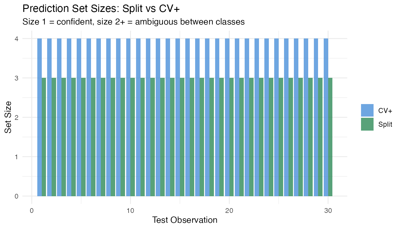
Practical Guidance
Which Method Should I Use?
| Scenario | Recommendation | Why |
|---|---|---|
| Large dataset (), fast results needed | Split | 1 fit, strong guarantee |
| Small dataset () | CV+ | No data waste, tighter intervals |
| Need tightest possible intervals | Jackknife+ | LOO calibration, most precise |
| Model already trained (production) | Generic | 0 re-fits, heuristic only (no coverage guarantee) |
| Nonlinear relationship suspected | CV+ with fregre.np | Distribution-free + flexible model |
| Classification with few samples | CV+ classification | All data used for calibration |
Sample Size Requirements
-
Split conformal: rule of thumb:
(e.g.,
for
).
With
cal.fraction = 0.25and , you get 25 calibration points — sufficient for most cases. - CV+: effective with . All data contributes to both training and calibration.
- Jackknife+: most data-efficient but requires model fits. Practical for .
Computational Cost
| Method | Model fits | Relative cost |
|---|---|---|
| Split | 1 | Fastest |
| Generic | 0 (pre-fitted) | Fastest |
| CV+ (5-fold) | 5 | Moderate |
| Jackknife+ | Slowest |
Common Pitfalls
-
Too few calibration points: split conformal with
small
and small
cal.fractiongives noisy intervals. Use CV+ instead. -
Too many FPC components: overfitting the base model
produces optimistic residuals, widening conformal intervals. Use
model.selection.ncomp()to choosencomp. - Confusing coverage guarantees: split and generic give ; CV+ and jackknife+ give in theory but often achieve near- empirically.
-
Ignoring the base model: conformal guarantees
coverage regardless of model quality, but a better base model produces
tighter intervals. Always tune
ncompand consider bothfregre.lmandfregre.np.
See Also
-
vignette("articles/uncertainty-quantification")— detailed UQ with parametric intervals, LOO-CV, and bootstrap CI -
vignette("articles/conformal-classification")— in-depth classification conformal with scoring rules and classifier comparison -
vignette("articles/scalar-on-function")— base regression models
References
Vovk, V., Gammerman, A. and Shafer, G. (2005). Algorithmic Learning in a Random World. Springer.
Barber, R.F., Candes, E.J., Ramdas, A. and Tibshirani, R.J. (2021). Predictive inference with the jackknife+. Annals of Statistics, 49(1), 486–507.
Romano, Y., Patterson, E. and Candes, E. (2019). Conformalized quantile regression. Advances in Neural Information Processing Systems, 32.