Finding the Best Basis Representation

Introduction

Basis representation is fundamental in functional data analysis. Instead of working with raw observations at discrete points, we represent curves as linear combinations of basis functions:

$X(t) = \sum_{k=1}^{K} c_k B_k(t)$

where $B_k(t)$ are basis functions and $c_k$ are coefficients.

This approach provides:

Smoothing: Reduces noise by projecting onto a lower-dimensional space
Dimensionality reduction: Represents infinite-dimensional functions with finite coefficients
Regularization: Controls curve smoothness through basis choice and penalties

fdars provides tools to find the optimal basis representation for your data.

library(fdars)
#> 
#> Attaching package: 'fdars'
#> The following objects are masked from 'package:stats':
#> 
#>     cov, decompose, deriv, median, sd, var
#> The following object is masked from 'package:base':
#> 
#>     norm
library(ggplot2)
theme_set(theme_minimal())
set.seed(42)

Creating Example Data

Let’s create functional data with a known signal plus noise:

# Generate noisy functional data
t <- seq(0, 1, length.out = 100)
n <- 30  # number of curves

# True underlying signal: mixture of sin waves
true_signal <- function(t) sin(2 * pi * t) + 0.5 * sin(4 * pi * t)

# Generate noisy observations
X <- matrix(0, n, length(t))
for (i in 1:n) {
  X[i, ] <- true_signal(t) + rnorm(length(t), sd = 0.3)
}
fd <- fdata(X, argvals = t)

# Plot the data
plot(fd, alpha = 0.3)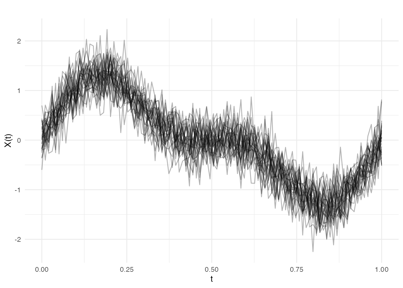

Choosing a Basis Type

fdars supports two main basis types:

B-splines (default)

Best for non-periodic data
Local support: each basis function is non-zero only in a limited region
Good for capturing local features
Computationally efficient

Fourier Basis

Best for periodic data (cycles, seasonal patterns)
Global support: each basis function spans the entire domain
Natural for data with harmonic structure

# Compare B-spline and Fourier representations
coefs_bspline <- fdata2basis(fd, nbasis = 15, type = "bspline")
coefs_fourier <- fdata2basis(fd, nbasis = 15, type = "fourier")

# Reconstruct
fd_bspline <- basis2fdata(coefs_bspline, argvals = t, type = "bspline")
fd_fourier <- basis2fdata(coefs_fourier, argvals = t, type = "fourier")

# Plot comparison for first curve
df_compare <- data.frame(
  t = rep(t, 3),
  value = c(fd$data[1, ], fd_bspline$data[1, ], fd_fourier$data[1, ]),
  type = factor(rep(c("Original", "B-spline (K=15)", "Fourier (K=15)"), each = length(t)),
                levels = c("Original", "B-spline (K=15)", "Fourier (K=15)"))
)

ggplot(df_compare, aes(x = t, y = value, color = type, linewidth = type)) +
  geom_line() +
  scale_color_manual(values = c("Original" = "gray50", "B-spline (K=15)" = "blue",
                                 "Fourier (K=15)" = "red")) +
  scale_linewidth_manual(values = c("Original" = 0.5, "B-spline (K=15)" = 1,
                                     "Fourier (K=15)" = 1)) +
  labs(x = "t", y = "X(t)", title = "Basis Representation Comparison") +
  theme(legend.position = "bottom", legend.title = element_blank()) +
  guides(linewidth = "none")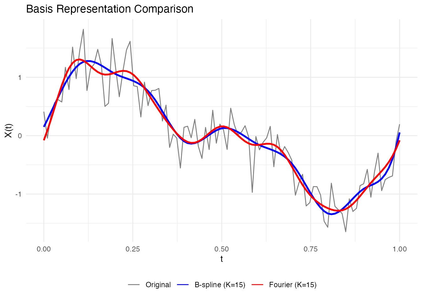

For our sinusoidal data, Fourier basis is more natural since the true signal is composed of sine waves.

Selecting the Number of Basis Functions

The key question: How many basis functions should we use?

Too few: Underfitting (misses important features)
Too many: Overfitting (fits noise)

Information Criteria

fdars provides three criteria to evaluate basis representations:

Criterion	Formula	Penalizes
GCV	$\frac{RSS/n}{(1 - edf/n)^2}$	Effective degrees of freedom
AIC	$n \log(RSS/n) + 2 \cdot edf$	Model complexity (moderate)
BIC	$n \log(RSS/n) + \log(n) \cdot edf$	Model complexity (strong)

# Compute criteria for different nbasis values
nbasis_range <- 5:25

gcv_scores <- sapply(nbasis_range, function(k) basis.gcv(fd, nbasis = k, type = "fourier"))
aic_scores <- sapply(nbasis_range, function(k) basis.aic(fd, nbasis = k, type = "fourier"))
bic_scores <- sapply(nbasis_range, function(k) basis.bic(fd, nbasis = k, type = "fourier"))

# Find optimal values
opt_gcv <- nbasis_range[which.min(gcv_scores)]
opt_aic <- nbasis_range[which.min(aic_scores)]
opt_bic <- nbasis_range[which.min(bic_scores)]

# Create data frame for plotting
df_criteria <- data.frame(
  nbasis = rep(nbasis_range, 3),
  score = c(gcv_scores, aic_scores, bic_scores),
  criterion = rep(c("GCV", "AIC", "BIC"), each = length(nbasis_range)),
  optimal = c(nbasis_range == opt_gcv, nbasis_range == opt_aic, nbasis_range == opt_bic)
)

df_optimal <- data.frame(
  criterion = c("GCV", "AIC", "BIC"),
  nbasis = c(opt_gcv, opt_aic, opt_bic)
)

ggplot(df_criteria, aes(x = nbasis, y = score)) +
  geom_line(color = "steelblue") +
  geom_point(color = "steelblue") +
  geom_vline(data = df_optimal, aes(xintercept = nbasis),
             linetype = "dashed", color = "red") +
  facet_wrap(~ criterion, scales = "free_y") +
  labs(x = "Number of basis functions", y = "Score",
       title = "Information Criteria for Basis Selection") +
  theme_minimal()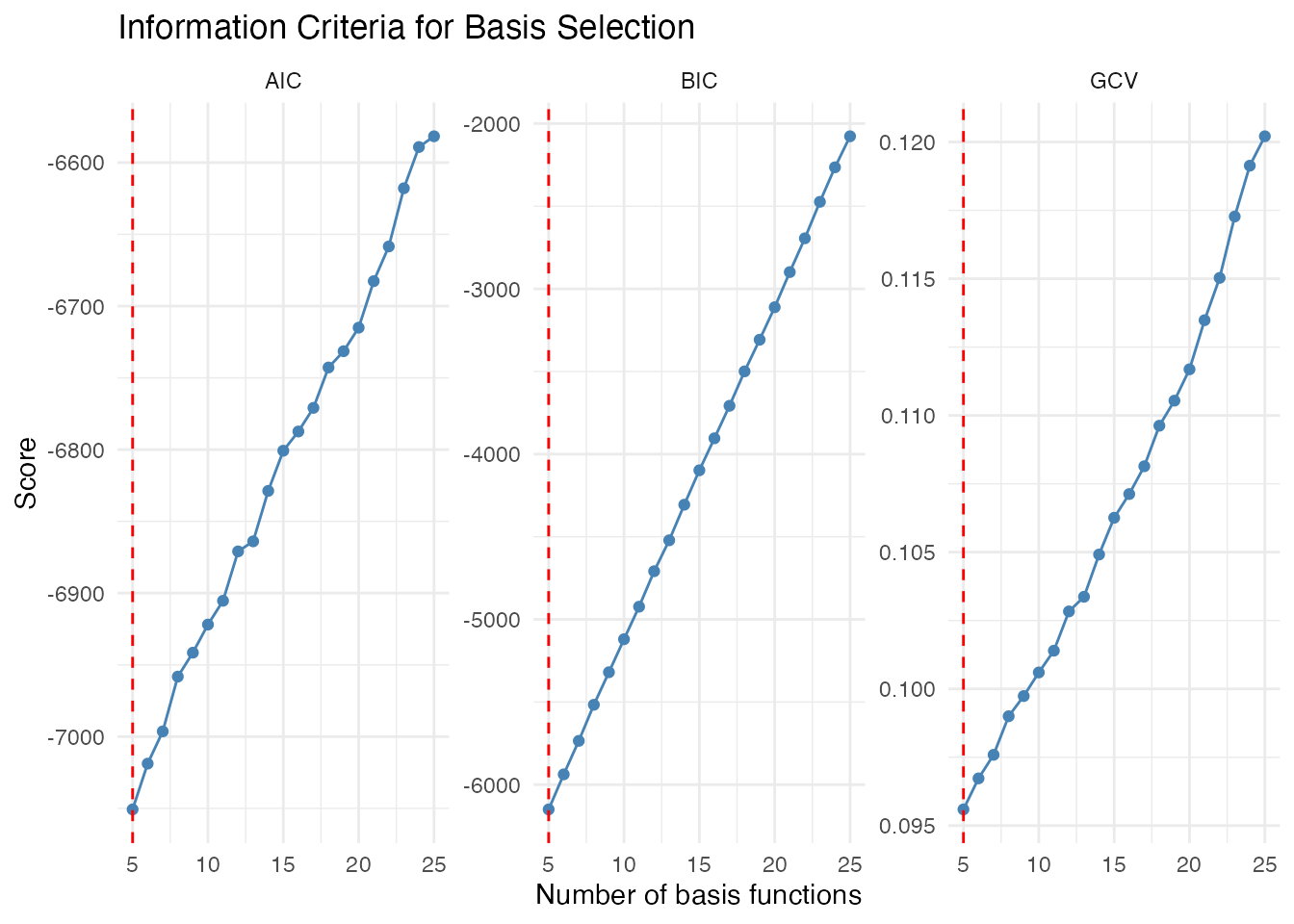


cat("Optimal nbasis - GCV:", opt_gcv, "\n")
#> Optimal nbasis - GCV: 5
cat("Optimal nbasis - AIC:", opt_aic, "\n")
#> Optimal nbasis - AIC: 5
cat("Optimal nbasis - BIC:", opt_bic, "\n")
#> Optimal nbasis - BIC: 5

Interpretation:

GCV (Generalized Cross-Validation): Often a good default, balances fit and complexity
AIC: Tends to select slightly more complex models
BIC: More conservative, penalizes complexity more strongly for larger samples

Complex Signal Example: B-spline vs Fourier

The previous example used a sinusoidal signal which is ideally suited for Fourier basis. Let’s now consider a complex non-periodic signal that’s better suited for B-splines:

# Generate data with non-periodic features
set.seed(123)
t2 <- seq(0, 1, length.out = 100)
n2 <- 30

# Complex signal: polynomial trend + localized bump
complex_signal <- function(t) {
  trend <- 2 * t^2 - t
  bump <- 0.8 * exp(-((t - 0.3)^2) / (2 * 0.05^2))
  sharp <- 0.5 * sqrt(pmax(0, t - 0.7))
  trend + bump + sharp
}

X2 <- matrix(0, n2, length(t2))
for (i in 1:n2) {
  X2[i, ] <- complex_signal(t2) + rnorm(length(t2), sd = 0.15)
}
fd2 <- fdata(X2, argvals = t2)

# Plot the raw complex signal data
plot(fd2) +
  labs(title = "Complex Signal: Polynomial Trend + Gaussian Bump + Sharp Edge",
       x = "t", y = "Value")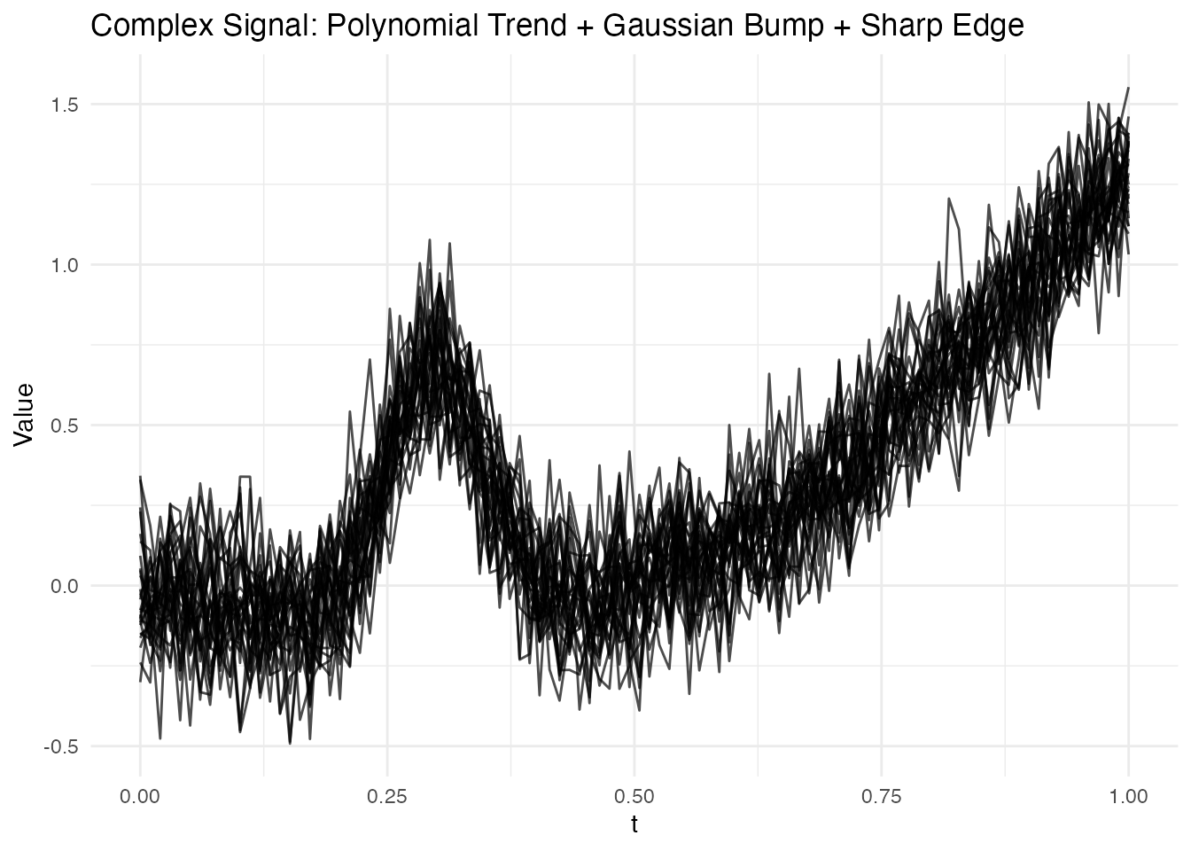

This signal has three distinct features that challenge different basis types:

Polynomial trend: Smooth, spanning the full domain
Gaussian bump at $t=0.3$ : A localized feature
Sharp edge at $t=0.7$ : A non-smooth transition

Let’s see which basis type handles this better:

# Compare B-spline vs Fourier for this data
nbasis_range <- 5:25

# B-spline criteria
gcv_bspline <- sapply(nbasis_range, function(k) basis.gcv(fd2, nbasis = k, type = "bspline"))
aic_bspline <- sapply(nbasis_range, function(k) basis.aic(fd2, nbasis = k, type = "bspline"))

# Fourier criteria
gcv_fourier <- sapply(nbasis_range, function(k) basis.gcv(fd2, nbasis = k, type = "fourier"))
aic_fourier <- sapply(nbasis_range, function(k) basis.aic(fd2, nbasis = k, type = "fourier"))

# Find optimal nbasis for each type
opt_bspline <- nbasis_range[which.min(gcv_bspline)]
opt_fourier <- nbasis_range[which.min(gcv_fourier)]

cat("Optimal B-spline nbasis:", opt_bspline, "(GCV:", round(min(gcv_bspline), 4), ")\n")
#> Optimal B-spline nbasis: 15 (GCV: 0.0259 )
cat("Optimal Fourier nbasis:", opt_fourier, "(GCV:", round(min(gcv_fourier), 4), ")\n")
#> Optimal Fourier nbasis: 14 (GCV: 0.048 )
cat("\nB-spline wins with", round((1 - min(gcv_bspline)/min(gcv_fourier)) * 100, 1),
    "% lower GCV score\n")
#> 
#> B-spline wins with 46.1 % lower GCV score

# Create comparison plot - use SAME scale to show B-spline advantage
df_gcv <- data.frame(
  nbasis = rep(nbasis_range, 2),
  GCV = c(gcv_bspline, gcv_fourier),
  basis = rep(c("B-spline", "Fourier"), each = length(nbasis_range))
)

ggplot(df_gcv, aes(x = nbasis, y = GCV, color = basis)) +
  geom_line(linewidth = 1) +
  geom_point(size = 2) +
  geom_hline(yintercept = min(gcv_bspline), linetype = "dashed",
             color = "steelblue", alpha = 0.5) +
  geom_hline(yintercept = min(gcv_fourier), linetype = "dashed",
             color = "coral", alpha = 0.5) +
  annotate("text", x = 24, y = min(gcv_bspline), label = "B-spline optimum",
           vjust = -0.5, hjust = 1, size = 3, color = "steelblue") +
  annotate("text", x = 24, y = min(gcv_fourier), label = "Fourier optimum",
           vjust = 1.5, hjust = 1, size = 3, color = "coral") +
  labs(x = "Number of basis functions", y = "GCV Score (lower is better)",
       title = "GCV Comparison: B-spline vs Fourier for Non-Periodic Signal",
       subtitle = "B-spline clearly outperforms Fourier for this complex signal") +
  scale_color_manual(values = c("B-spline" = "steelblue", "Fourier" = "coral")) +
  theme(legend.position = "bottom")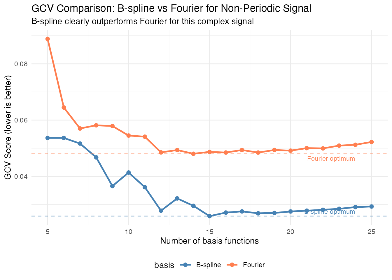

Important: Note that both curves are plotted on the same scale. The B-spline basis achieves a substantially lower GCV score, confirming it’s the better choice for this non-periodic signal with localized features.

Now let’s visualize how each optimal basis representation captures the complex signal:

# Fit both bases at their optimal values
coefs_bspline <- fdata2basis(fd2, nbasis = opt_bspline, type = "bspline")
coefs_fourier <- fdata2basis(fd2, nbasis = opt_fourier, type = "fourier")
fitted_bspline <- basis2fdata(coefs_bspline, argvals = t2, type = "bspline")
fitted_fourier <- basis2fdata(coefs_fourier, argvals = t2, type = "fourier")

# Plot comparison for one curve
i <- 1
df_fit <- data.frame(
  t = rep(t2, 4),
  value = c(fd2$data[i, ], complex_signal(t2),
            fitted_bspline$data[i, ], fitted_fourier$data[i, ]),
  type = factor(rep(c("Observed (noisy)", "True signal",
                      paste0("B-spline (K=", opt_bspline, ")"),
                      paste0("Fourier (K=", opt_fourier, ")")), each = length(t2)),
                levels = c("Observed (noisy)", "True signal",
                           paste0("B-spline (K=", opt_bspline, ")"),
                           paste0("Fourier (K=", opt_fourier, ")")))
)

ggplot(df_fit, aes(x = t, y = value, color = type, linetype = type, linewidth = type)) +
  geom_line() +
  scale_color_manual(values = c("Observed (noisy)" = "gray70",
                                 "True signal" = "black",
                                 setNames("steelblue", paste0("B-spline (K=", opt_bspline, ")")),
                                 setNames("coral", paste0("Fourier (K=", opt_fourier, ")")))) +
  scale_linetype_manual(values = c("Observed (noisy)" = "solid",
                                    "True signal" = "dashed",
                                    setNames("solid", paste0("B-spline (K=", opt_bspline, ")")),
                                    setNames("solid", paste0("Fourier (K=", opt_fourier, ")")))) +
  scale_linewidth_manual(values = c("Observed (noisy)" = 0.4,
                                     "True signal" = 1,
                                     setNames(1, paste0("B-spline (K=", opt_bspline, ")")),
                                     setNames(1, paste0("Fourier (K=", opt_fourier, ")")))) +
  labs(x = "t", y = "Value", color = NULL, linetype = NULL,
       title = "Basis Representation Comparison: B-spline vs Fourier",
       subtitle = "B-spline captures localized features; Fourier shows ringing artifacts") +
  theme(legend.position = "bottom") +
  guides(linewidth = "none")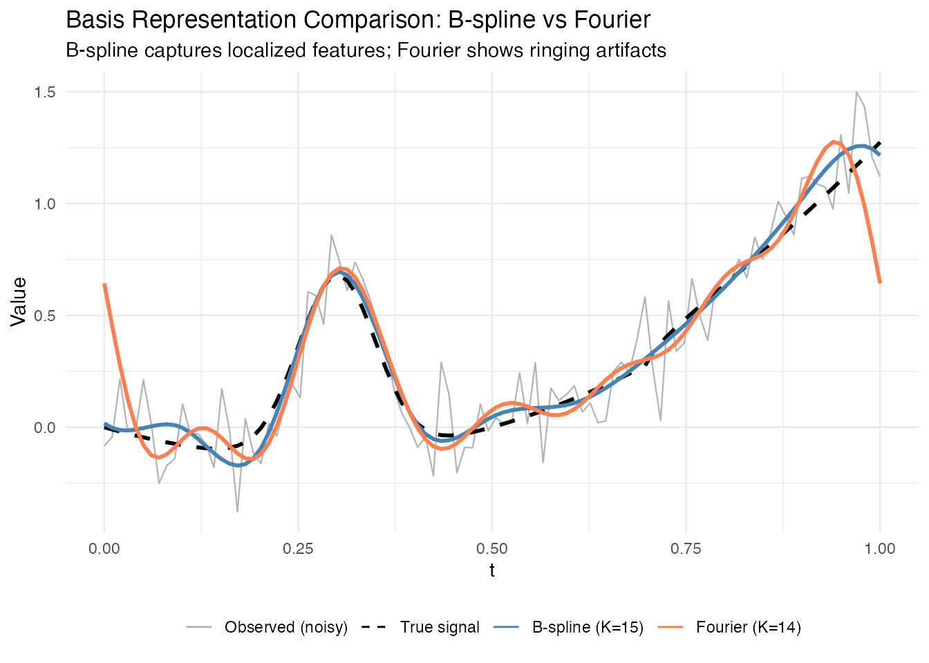

Key observations:

B-splines are better for localized features (like the Gaussian bump)
Fourier basis needs more functions to approximate non-periodic signals
Information criteria help select both basis type AND number of functions

Automatic Selection with `fdata2basis_cv()`

For convenience, use fdata2basis_cv() to automatically find the optimal number of basis functions:

# Automatic selection using GCV
cv_result <- fdata2basis_cv(fd, nbasis.range = 5:25, type = "fourier", criterion = "GCV")
print(cv_result)
#> Basis Cross-Validation Results
#> ==============================
#> Criterion: GCV 
#> Optimal nbasis: 5 
#> Score at optimal: 0.09559293 
#> Range tested: 5 - 25

# Visualize the selection
plot(cv_result)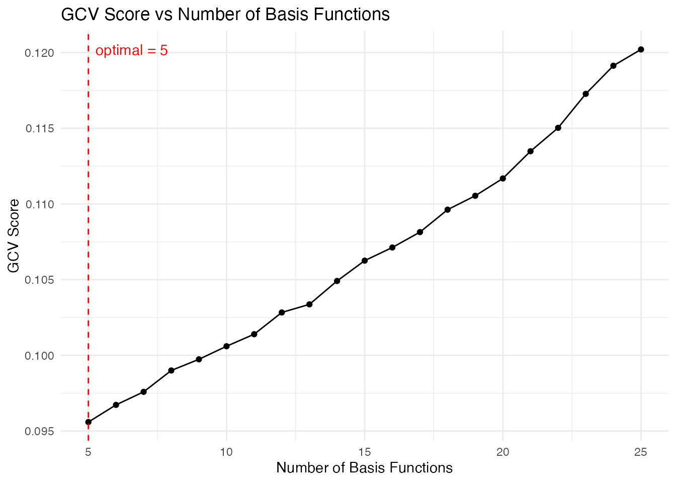

The function returns the optimal number of basis functions and the fitted curves:

# Plot the smoothed data
plot(cv_result$fitted, alpha = 0.5, main = paste("Smoothed with", cv_result$optimal.nbasis, "Fourier basis"))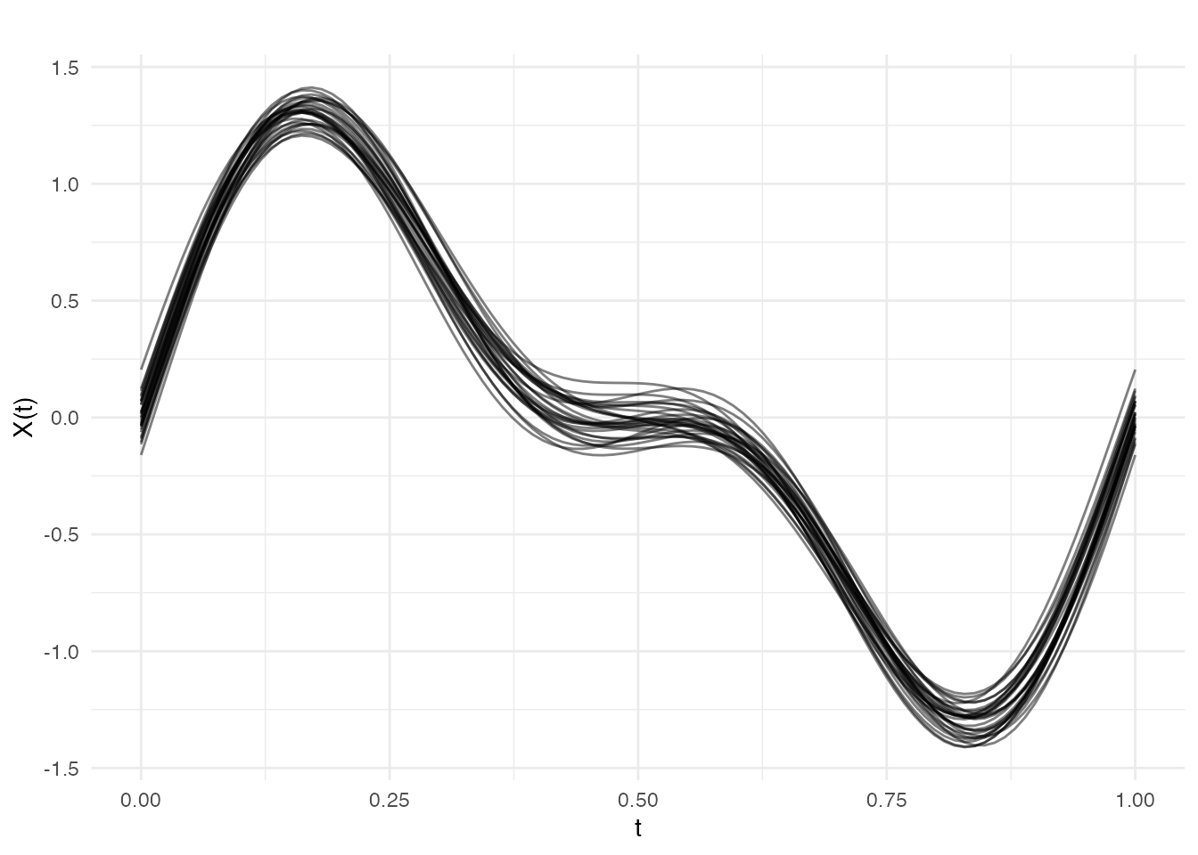

K-fold Cross-Validation

For a more robust estimate, use k-fold cross-validation:

# K-fold cross-validation (slower but more robust)
cv_kfold <- fdata2basis_cv(fd, nbasis.range = 5:25, type = "fourier",
                            criterion = "CV", kfold = 10)
print(cv_kfold$optimal.nbasis)

P-spline Smoothing

P-splines (Penalized B-splines) offer an alternative approach: instead of selecting the number of basis functions, we use many basis functions but add a roughness penalty:

$\text{minimize} \quad ||y - Bc||^2 + \lambda c' D' D c$

where: - $B$ is the B-spline basis matrix - $c$ are coefficients - $D$ is a difference matrix (controls smoothness) - $\lambda$ is the penalty parameter

# Fit P-spline with fixed lambda
result_fixed <- pspline(fd[1], nbasis = 25, lambda = 10)
print(result_fixed)
#> P-spline Smoothing Results
#> ==========================
#> Number of curves: 1 
#> Number of basis functions: 25 
#> Penalty order: 2 
#> Lambda: 1e+01 
#> Effective df: 6.68 
#> GCV: 1.151e-01

# Compare different lambda values
lambdas <- c(0.01, 1, 100, 10000)
df_lambda <- do.call(rbind, lapply(lambdas, function(lam) {
  result <- pspline(fd[1], nbasis = 25, lambda = lam)
  data.frame(
    t = rep(t, 2),
    value = c(fd$data[1, ], result$fdata$data[1, ]),
    type = rep(c("Original", "Smoothed"), each = length(t)),
    lambda = paste("lambda =", lam)
  )
}))
df_lambda$lambda <- factor(df_lambda$lambda, levels = paste("lambda =", lambdas))

ggplot(df_lambda, aes(x = t, y = value, color = type, linewidth = type)) +
  geom_line() +
  scale_color_manual(values = c("Original" = "gray50", "Smoothed" = "blue")) +
  scale_linewidth_manual(values = c("Original" = 0.5, "Smoothed" = 1)) +
  facet_wrap(~ lambda, ncol = 2) +
  labs(x = "t", y = "X(t)", title = "P-spline Smoothing with Different Lambda") +
  theme_minimal() +
  theme(legend.position = "bottom", legend.title = element_blank())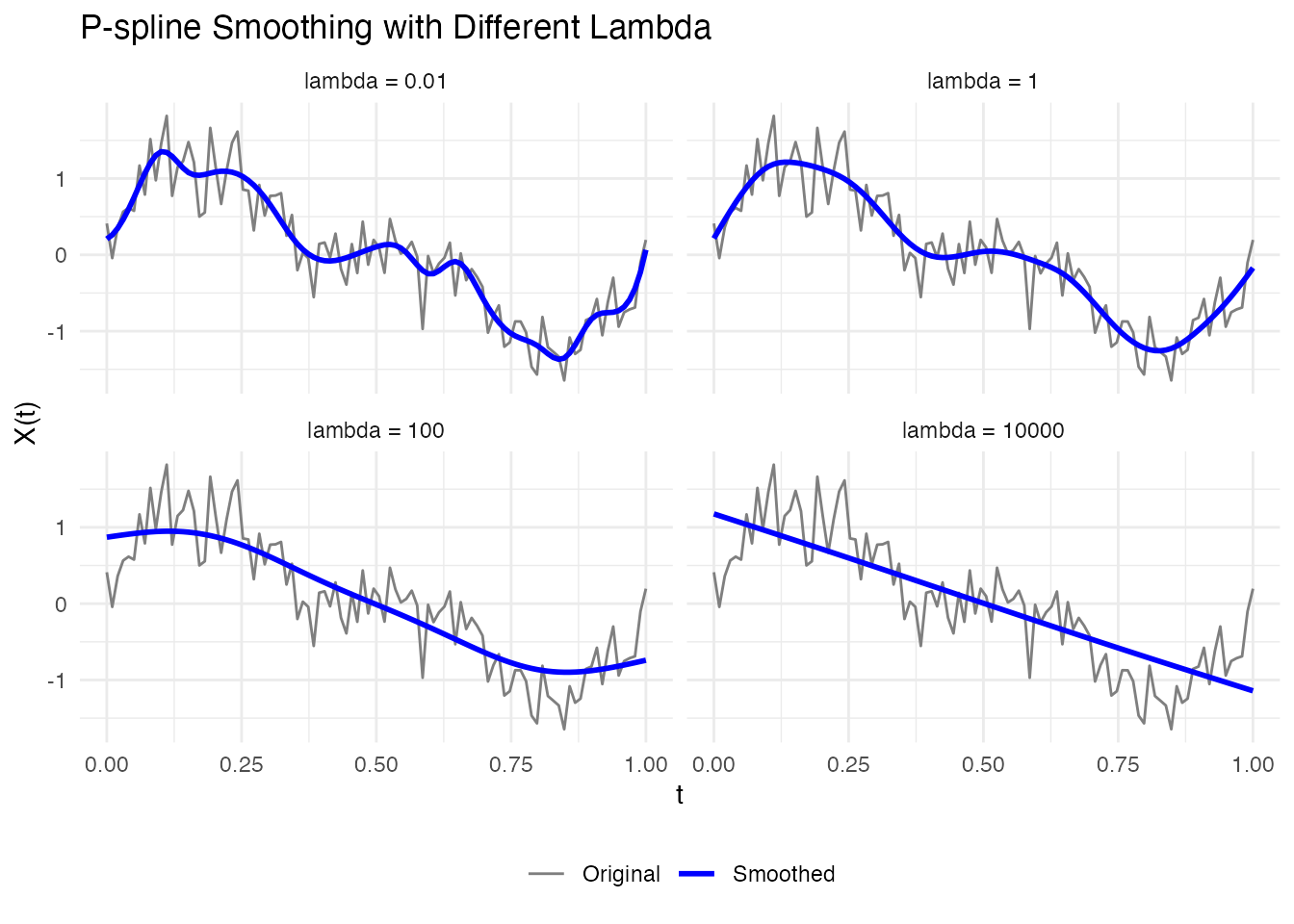

Automatic Lambda Selection

P-splines can automatically select the optimal smoothing parameter:

# Automatic lambda selection using GCV
result_auto <- pspline(fd[1], nbasis = 25, lambda.select = TRUE, criterion = "GCV")
cat("Selected lambda:", result_auto$lambda, "\n")
#> Selected lambda: 1.206793
cat("Effective df:", round(result_auto$edf, 2), "\n")
#> Effective df: 9.99

# Plot result
df_auto <- data.frame(
  t = rep(t, 3),
  value = c(fd$data[1, ], result_auto$fdata$data[1, ], true_signal(t)),
  type = factor(c(rep("Observed", length(t)),
                  rep("P-spline", length(t)),
                  rep("True signal", length(t))),
                levels = c("Observed", "P-spline", "True signal"))
)

ggplot(df_auto, aes(x = t, y = value, color = type, linetype = type, linewidth = type)) +
  geom_line() +
  scale_color_manual(values = c("Observed" = "gray50", "P-spline" = "blue",
                                 "True signal" = "red")) +
  scale_linetype_manual(values = c("Observed" = "solid", "P-spline" = "solid",
                                    "True signal" = "dashed")) +
  scale_linewidth_manual(values = c("Observed" = 0.5, "P-spline" = 1, "True signal" = 1)) +
  labs(x = "t", y = "X(t)", title = "P-spline with Auto-selected Lambda") +
  theme_minimal() +
  theme(legend.position = "bottom", legend.title = element_blank())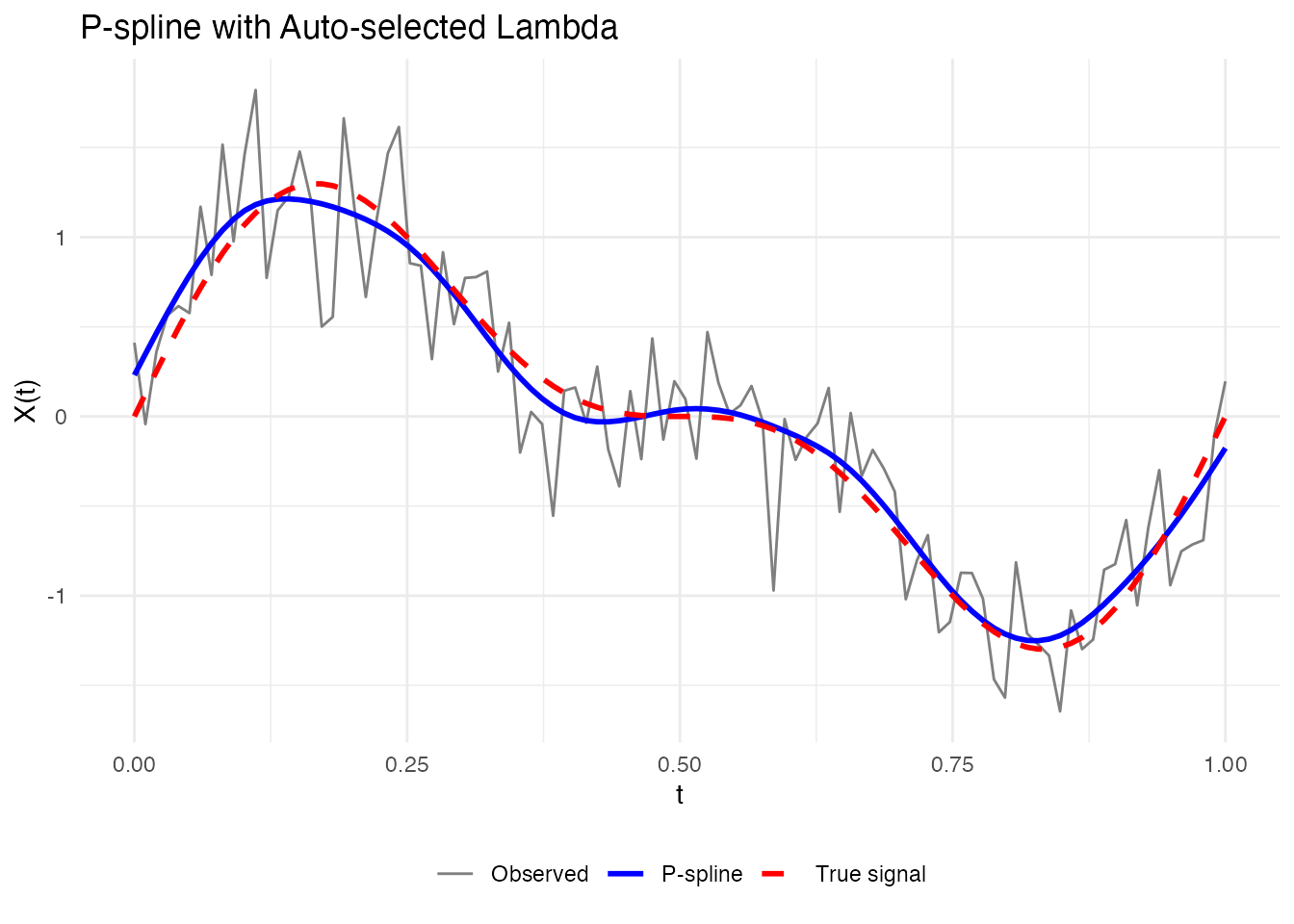

Smoothing Multiple Curves

P-splines work curve-by-curve, so you can smooth entire datasets:

# Smooth all curves with automatic lambda selection
result_all <- pspline(fd, nbasis = 25, lambda.select = TRUE)

# Plot smoothed data
plot(result_all$fdata, alpha = 0.5, main = "All curves smoothed with P-splines")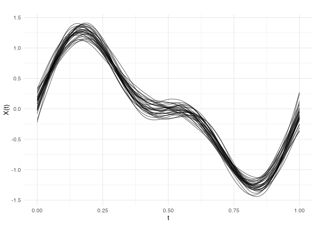

Comparing Approaches

Let’s compare the different smoothing approaches:

# Original noisy data
fd_single <- fd[1]

# 1. Simple basis projection (Fourier)
coefs <- fdata2basis(fd_single, nbasis = 9, type = "fourier")
fd_fourier <- basis2fdata(coefs, argvals = t, type = "fourier")

# 2. Optimal basis via CV
cv_opt <- fdata2basis_cv(fd_single, nbasis.range = 5:20, type = "fourier")
fd_cv <- cv_opt$fitted

# 3. P-spline with automatic lambda
ps_result <- pspline(fd_single, nbasis = 25, lambda.select = TRUE)
fd_pspline <- ps_result$fdata

# Plot comparison
df_comp <- data.frame(
  t = rep(t, 5),
  value = c(fd_single$data[1, ], fd_fourier$data[1, ], fd_cv$data[1, ],
            fd_pspline$data[1, ], true_signal(t)),
  method = factor(c(rep("Observed", length(t)),
                    rep("Fourier (K=9)", length(t)),
                    rep(paste0("CV-optimal (K=", cv_opt$optimal.nbasis, ")"), length(t)),
                    rep("P-spline", length(t)),
                    rep("True signal", length(t))),
                  levels = c("Observed", "Fourier (K=9)",
                             paste0("CV-optimal (K=", cv_opt$optimal.nbasis, ")"),
                             "P-spline", "True signal"))
)

ggplot(df_comp, aes(x = t, y = value, color = method, linetype = method, linewidth = method)) +
  geom_line() +
  scale_color_manual(values = c("Observed" = "gray50", "Fourier (K=9)" = "blue",
                                 "CV-optimal (K=9)" = "green", "P-spline" = "purple",
                                 "True signal" = "red",
                                 setNames("green", paste0("CV-optimal (K=", cv_opt$optimal.nbasis, ")")))) +
  scale_linetype_manual(values = c("Observed" = "solid", "Fourier (K=9)" = "solid",
                                    "CV-optimal (K=9)" = "solid", "P-spline" = "solid",
                                    "True signal" = "dashed",
                                    setNames("solid", paste0("CV-optimal (K=", cv_opt$optimal.nbasis, ")")))) +
  scale_linewidth_manual(values = c("Observed" = 0.5, "Fourier (K=9)" = 1,
                                     "CV-optimal (K=9)" = 1, "P-spline" = 1,
                                     "True signal" = 1,
                                     setNames(1, paste0("CV-optimal (K=", cv_opt$optimal.nbasis, ")")))) +
  labs(x = "t", y = "X(t)", title = "Comparison of Smoothing Methods", color = NULL) +
  theme_minimal() +
  theme(legend.position = "bottom") +
  guides(linetype = "none", linewidth = "none")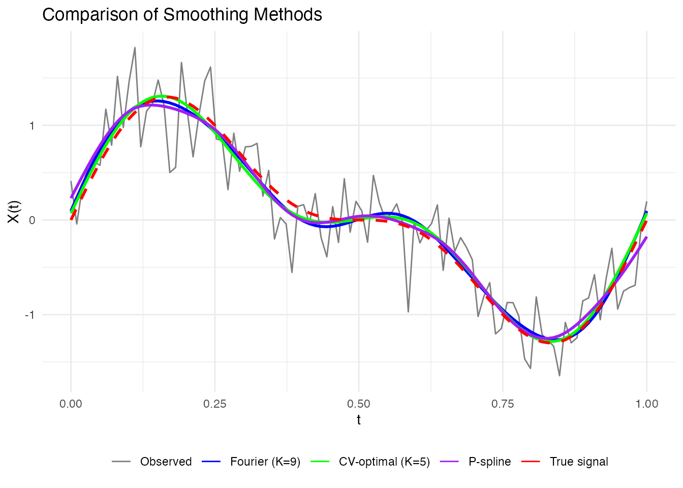

Recommendations

Situation	Recommended Approach
Periodic data	Fourier basis with GCV selection
Non-periodic data	B-spline basis with GCV selection
Heavy noise	P-splines with automatic lambda
Fast processing needed	Simple basis with fixed K
Publication-quality	K-fold CV for robust selection

Summary

Choose basis type based on data characteristics:
- Fourier for periodic patterns
- B-splines for non-periodic data
Select complexity using information criteria:
- fdata2basis_cv() for automatic nbasis selection
- basis.gcv(), basis.aic(), basis.bic() for manual comparison
Consider P-splines for:
- Heavy noise scenarios
- When you want smooth derivatives
- Automatic smoothing parameter selection
Validate by comparing reconstructed curves to the original data

References

Ramsay, J.O. and Silverman, B.W. (2005). Functional Data Analysis. Springer.
Eilers, P.H.C. and Marx, B.D. (1996). Flexible smoothing with B-splines and penalties. Statistical Science, 11(2), 89-121.