Distance Metrics and Semimetrics

Introduction

Distance measures are fundamental to many FDA methods including clustering, k-nearest neighbors regression, and outlier detection. fdars provides both true metrics (satisfying the triangle inequality) and semimetrics (which may not).

A metric $d$ on a space $\mathcal{X}$ satisfies:

1. $d(f, g) \geq 0$ (non-negativity)
2. $d(f, g) = 0 \Leftrightarrow f = g$ (identity of indiscernibles)
3. $d(f, g) = d(g, f)$ (symmetry)
4. $d(f, h) \leq d(f, g) + d(g, h)$ (triangle inequality)

A semimetric satisfies only conditions 1-3.

library(fdars)
#> 
#> Attaching package: 'fdars'
#> The following objects are masked from 'package:stats':
#> 
#>     cov, decompose, deriv, median, sd, var
#> The following object is masked from 'package:base':
#> 
#>     norm
library(ggplot2)
theme_set(theme_minimal())

# Create example data with different curve types
set.seed(42)
m <- 100
t_grid <- seq(0, 1, length.out = m)

# Four types of curves
curve1 <- sin(2 * pi * t_grid)                    # Sine
curve2 <- sin(2 * pi * t_grid + 0.5)              # Phase-shifted sine
curve3 <- cos(2 * pi * t_grid)                    # Cosine
curve4 <- sin(4 * pi * t_grid)                    # Higher frequency

X <- rbind(curve1, curve2, curve3, curve4)
fd <- fdata(X, argvals = t_grid,
            names = list(main = "Four Curve Types"))
plot(fd)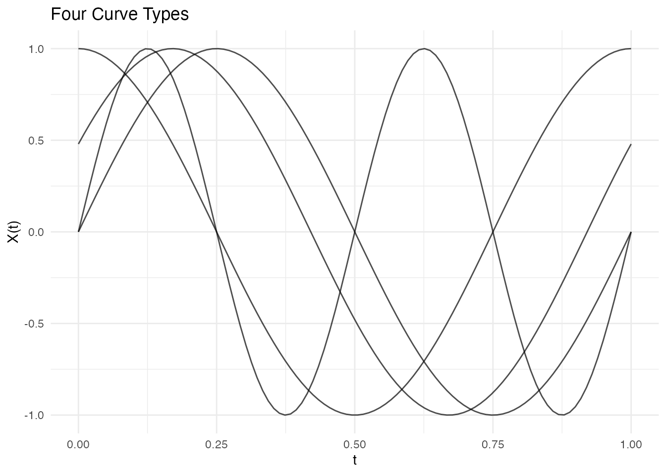

True Metrics

Lp Distance (metric.lp)

The $L^p$ distance is the most common choice for functional data. It computes the integrated $L^p$ norm of the difference between two functions:

$$d_p(f, g) = \left( \int_{\mathcal{T}} |f(t) - g(t)|^p \, dt \right)^{1/p}$$

For discrete observations, this is approximated using numerical integration (Simpson’s rule):

$$d_p(f, g) \approx \left( \sum_{j=1}^{m} w_j |f(t_j) - g(t_j)|^p \right)^{1/p}$$

where $w_j$ are quadrature weights.

Special cases:

• $p = 2$ (L2/Euclidean): Most common, corresponds to the standard functional norm. Sensitive to vertical differences.
• $p = 1$ (L1/Manhattan): More robust to outliers than L2.
• $p = \infty$ (L-infinity/Chebyshev): Maximum absolute difference, $d_\infty(f, g) = \max_t |f(t) - g(t)|$.

# L2 (Euclidean) distance - default
dist_l2 <- metric.lp(fd)
print(round(as.matrix(dist_l2), 3))
#>        curve1 curve2 curve3 curve4
#> curve1   0.00  0.350  1.000      1
#> curve2   0.35  0.000  0.722      1
#> curve3   1.00  0.722  0.000      1
#> curve4   1.00  1.000  1.000      0

# L1 (Manhattan) distance
dist_l1 <- metric.lp(fd, lp = 1)

# L-infinity (maximum) distance
dist_linf <- metric.lp(fd, lp = Inf)

Weighted Lp Distance

Apply different weights to different parts of the domain:

$$d_{p,w}(f, g) = \left( \int_{\mathcal{T}} w(t) |f(t) - g(t)|^p \, dt \right)^{1/p}$$

This is useful when certain parts of the domain are more important than others.

# Weight emphasizing the middle of the domain
w <- dnorm(t_grid, mean = 0.5, sd = 0.2)
w <- w / sum(w) * length(w)  # Normalize

dist_weighted <- metric.lp(fd, lp = 2, w = w)

Hausdorff Distance (metric.hausdorff)

The Hausdorff distance treats curves as sets of points $(t, f(t))$ in 2D space and computes the maximum of minimum distances:

$$d_H(f, g) = \max\left\{ \sup_{t \in \mathcal{T}} \inf_{s \in \mathcal{T}} \|P_f(t) - P_g(s)\|, \sup_{s \in \mathcal{T}} \inf_{t \in \mathcal{T}} \|P_f(t) - P_g(s)\| \right\}$$

where $P_f(t) = (t, f(t))$ is the point on the graph of $f$ at time $t$.

The Hausdorff distance is useful when:

• Curves may cross each other
• The timing of features is less important than their shape
• Comparing curves with different supports

dist_haus <- metric.hausdorff(fd)
print(round(as.matrix(dist_haus), 3))
#>        curve1 curve2 curve3 curve4
#> curve1  0.000  0.479  0.678  0.328
#> curve2  0.479  0.000  0.521  0.416
#> curve3  0.678  0.521  0.000  0.352
#> curve4  0.328  0.416  0.352  0.000

Dynamic Time Warping (metric.DTW)

DTW allows for non-linear alignment of curves before computing the distance. It finds the optimal warping path $\pi$ that minimizes:

$$d_{DTW}(f, g) = \min_{\pi} \sqrt{\sum_{(i,j) \in \pi} |f(t_i) - g(t_j)|^2}$$

subject to boundary conditions, monotonicity, and continuity constraints.

The Sakoe-Chiba band constraint limits the warping to $|i - j| \leq w$, preventing excessive distortion:

$$d_{DTW}^{SC}(f, g) = \min_{\pi: |i-j| \leq w} \sqrt{\sum_{(i,j) \in \pi} |f(t_i) - g(t_j)|^2}$$

DTW is particularly effective for:

• Phase-shifted signals
• Time series with varying speed
• Comparing signals with local time distortions

dist_dtw <- metric.DTW(fd)
print(round(as.matrix(dist_dtw), 3))
#>        curve1 curve2 curve3 curve4
#> curve1  0.000  1.452 18.185 24.844
#> curve2  1.452  0.000  3.488 25.980
#> curve3 18.185  3.488  0.000 40.825
#> curve4 24.844 25.980 40.825  0.000

Notice that DTW gives a smaller distance between the original sine and phase-shifted sine compared to L2, because it can align them:

# Compare L2 vs DTW for phase-shifted curves
cat("L2 distance (sine vs phase-shifted):", round(as.matrix(dist_l2)[1, 2], 3), "\n")
#> L2 distance (sine vs phase-shifted): 0.35
cat("DTW distance (sine vs phase-shifted):", round(as.matrix(dist_dtw)[1, 2], 3), "\n")
#> DTW distance (sine vs phase-shifted): 1.452

DTW with band constraint:

# Restrict warping to 10% of the series length
dist_dtw_band <- metric.DTW(fd, w = round(m * 0.1))

Kullback-Leibler Divergence (metric.kl)

The symmetric Kullback-Leibler divergence treats normalized curves as probability density functions:

$$d_{KL}(f, g) = \frac{1}{2}\left[ \int f(t) \log\frac{f(t)}{g(t)} \, dt + \int g(t) \log\frac{g(t)}{f(t)} \, dt \right]$$

Before computing, curves are shifted to be non-negative and normalized to integrate to 1:

$$\tilde{f}(t) = \frac{f(t) - \min_s f(s) + \epsilon}{\int [f(s) - \min_s f(s) + \epsilon] \, ds}$$

This metric is useful for:

• Comparing density-like functions
• Distribution comparison
• Information-theoretic analysis

# Shift curves to be positive for KL
X_pos <- X - min(X) + 0.1
fd_pos <- fdata(X_pos, argvals = t_grid)

dist_kl <- metric.kl(fd_pos)
print(round(as.matrix(dist_kl), 3))
#>        curve1 curve2 curve3 curve4
#> curve1  0.000  0.139  1.208  1.187
#> curve2  0.139  0.000  0.630  1.426
#> curve3  1.208  0.630  0.000  1.156
#> curve4  1.187  1.426  1.156  0.000

Semimetrics

Semimetrics may not satisfy the triangle inequality but can be more appropriate for certain applications or provide computational advantages.

PCA-Based Semimetric (semimetric.pca)

Projects curves onto the first $q$ principal components and computes the Euclidean distance in the reduced space:

$$d_{PCA}(f, g) = \sqrt{\sum_{k=1}^{q} (\xi_k^f - \xi_k^g)^2}$$

where $\xi_k^f = \langle f - \bar{f}, \phi_k \rangle$ is the $k$-th principal component score of $f$, and $\phi_k$ are the eigenfunctions from functional PCA.

This semimetric is useful for:

• Dimension reduction before distance computation
• Noise reduction (low-rank approximation)
• Computational efficiency with many evaluation points

# Distance using first 3 PCs
dist_pca <- semimetric.pca(fd, ncomp = 3)
print(round(as.matrix(dist_pca), 3))
#>        [,1]  [,2]   [,3]   [,4]
#> [1,]  0.000 3.514 10.000  9.950
#> [2,]  3.514 0.000  7.198  9.961
#> [3,] 10.000 7.198  0.000 10.000
#> [4,]  9.950 9.961 10.000  0.000

Derivative-Based Semimetric (semimetric.deriv)

Computes the $L^p$ distance based on the $r$-th derivative of the curves:

$$d_{deriv}^{(r)}(f, g) = \left( \int_{\mathcal{T}} |f^{(r)}(t) - g^{(r)}(t)|^p \, dt \right)^{1/p}$$

where $f^{(r)}$ denotes the $r$-th derivative of $f$.

This semimetric focuses on the shape and dynamics of curves rather than their absolute values. It is particularly useful when:

• Comparing rate of change (first derivative)
• Analyzing curvature (second derivative)
• Functions are measured with different baselines

# First derivative (velocity)
dist_deriv1 <- semimetric.deriv(fd, nderiv = 1)

# Second derivative (acceleration/curvature)
dist_deriv2 <- semimetric.deriv(fd, nderiv = 2)

cat("First derivative distances:\n")
#> First derivative distances:
print(round(as.matrix(dist_deriv1), 3))
#>       [,1]  [,2]  [,3]  [,4]
#> [1,] 0.000 2.197 6.279 9.912
#> [2,] 2.197 0.000 4.530 9.912
#> [3,] 6.279 4.530 0.000 9.912
#> [4,] 9.912 9.912 9.912 0.000

Basis Semimetric (semimetric.basis)

Projects curves onto a basis (B-spline or Fourier) and computes the Euclidean distance between the coefficient vectors:

$$d_{basis}(f, g) = \|c^f - c^g\|_2 = \sqrt{\sum_{k=1}^{K} (c_k^f - c_k^g)^2}$$

where $c^f = (c_1^f, \ldots, c_K^f)$ are the basis coefficients from $f(t) \approx \sum_{k=1}^{K} c_k^f B_k(t)$.

For B-splines: Local support provides good approximation of local features.

For Fourier basis: Global support captures periodic patterns efficiently.

# B-spline basis (local features)
dist_bspline <- semimetric.basis(fd, nbasis = 15, basis = "bspline")

# Fourier basis (periodic patterns)
dist_fourier <- semimetric.basis(fd, nbasis = 11, basis = "fourier")

cat("B-spline basis distances:\n")
#> B-spline basis distances:
print(round(as.matrix(dist_bspline), 3))
#>       [,1]  [,2]  [,3]  [,4]
#> [1,] 0.000 1.509 4.015 3.913
#> [2,] 1.509 0.000 2.771 3.999
#> [3,] 4.015 2.771 0.000 4.289
#> [4,] 3.913 3.999 4.289 0.000

Fourier Semimetric (semimetric.fourier)

Uses the Fast Fourier Transform (FFT) to compute Fourier coefficients and measures distance based on the first $K$ frequency components:

$$d_{FFT}(f, g) = \sqrt{\sum_{k=0}^{K} |\hat{f}_k - \hat{g}_k|^2}$$

where $\hat{f}_k$ is the $k$-th Fourier coefficient computed via FFT.

This is computationally efficient for large datasets and particularly useful for periodic or frequency-domain analysis.

dist_fft <- semimetric.fourier(fd, nfreq = 5)
cat("Fourier (FFT) distances:\n")
#> Fourier (FFT) distances:
print(round(as.matrix(dist_fft), 3))
#>        curve1 curve2 curve3 curve4
#> curve1  0.000  0.005  0.012  0.694
#> curve2  0.005  0.000  0.008  0.695
#> curve3  0.012  0.008  0.000  0.700
#> curve4  0.694  0.695  0.700  0.000

Horizontal Shift Semimetric (semimetric.hshift)

Finds the optimal horizontal shift before computing the $L^2$ distance:

$$d_{hshift}(f, g) = \min_{|h| \leq h_{max}} \left( \int_{\mathcal{T}} |f(t) - g(t+h)|^2 \, dt \right)^{1/2}$$

where $h$ is the shift in discrete time units and $h_{max}$ is the maximum allowed shift.

This semimetric is simpler than DTW (only horizontal shifts, no warping) but can be very effective for:

• Phase-shifted periodic signals
• ECG or other physiological signals with timing variations
• Comparing curves where horizontal alignment is meaningful

dist_hshift <- semimetric.hshift(fd)
cat("Horizontal shift distances:\n")
#> Horizontal shift distances:
print(round(as.matrix(dist_hshift), 3))
#>        curve1 curve2 curve3 curve4
#> curve1  0.000  0.005  0.010  0.733
#> curve2  0.005  0.000  0.005  0.629
#> curve3  0.010  0.005  0.000  0.718
#> curve4  0.733  0.629  0.718  0.000

Unified Interface

Use metric() for a unified interface to all distance functions:

# Different methods via single function
d1 <- metric(fd, method = "lp", lp = 2)
d2 <- metric(fd, method = "dtw")
d3 <- metric(fd, method = "hausdorff")
d4 <- metric(fd, method = "pca", ncomp = 2)

Comparing Distance Measures

Different distance measures capture different aspects of curve similarity:

# Create comparison data
dists <- list(
  L2 = as.vector(as.matrix(dist_l2)),
  L1 = as.vector(as.matrix(dist_l1)),
  DTW = as.vector(as.matrix(dist_dtw)),
  Hausdorff = as.vector(as.matrix(dist_haus))
)

# Correlation between distance measures
dist_mat <- do.call(cbind, dists)
cat("Correlation between distance measures:\n")
#> Correlation between distance measures:
print(round(cor(dist_mat), 2))
#>             L2   L1  DTW Hausdorff
#> L2        1.00 1.00 0.82      0.74
#> L1        1.00 1.00 0.82      0.74
#> DTW       0.82 0.82 1.00      0.32
#> Hausdorff 0.74 0.74 0.32      1.00

Distance Matrices for Larger Samples

# Generate larger sample
set.seed(123)
n <- 50
X_large <- matrix(0, n, m)
for (i in 1:n) {
  phase <- runif(1, 0, 2*pi)
  freq <- sample(1:3, 1)
  X_large[i, ] <- sin(freq * pi * t_grid + phase) + rnorm(m, sd = 0.1)
}
fd_large <- fdata(X_large, argvals = t_grid)

# Compute distance matrix
dist_matrix <- metric.lp(fd_large)

# Visualize as heatmap using ggplot2
dist_df <- expand.grid(Curve1 = 1:n, Curve2 = 1:n)
dist_df$Distance <- as.vector(as.matrix(dist_matrix))

ggplot(dist_df, aes(x = Curve1, y = Curve2, fill = Distance)) +
  geom_tile() +
  scale_fill_viridis_c(option = "magma") +
  coord_equal() +
  labs(x = "Curve", y = "Curve", title = "L2 Distance Matrix") +
  theme_minimal()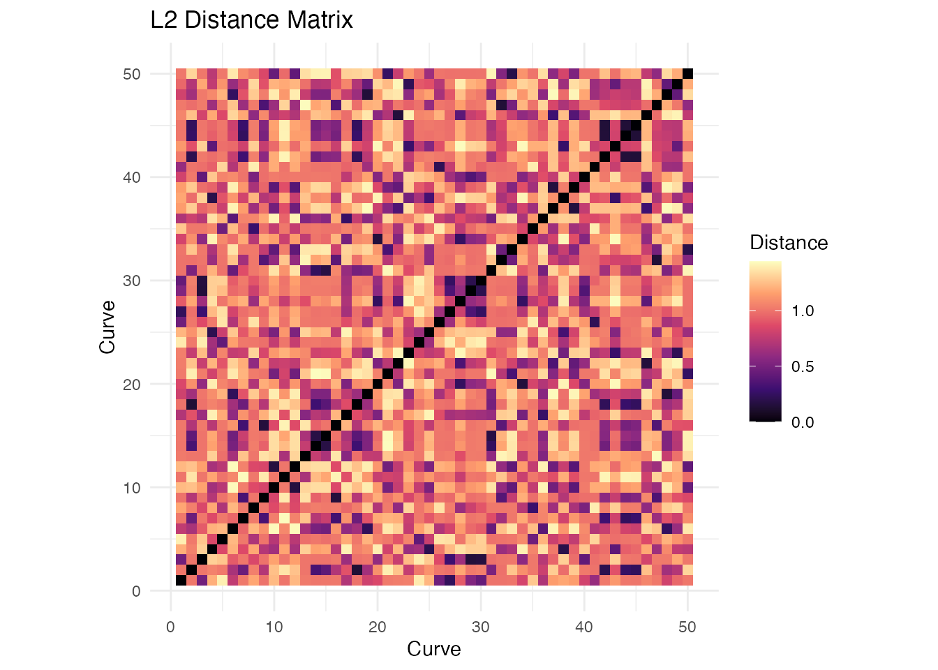

Metric Properties Summary

Distance	Type	Triangle Ineq.	Phase Invariant	Computational Cost
Lp	Metric	Yes	No	O(nm)
Hausdorff	Metric	Yes	Partial	O(nm²)
DTW	Metric*	Yes*	Yes	O(nm²)
KL	Semimetric	No	No	O(nm)
PCA	Semimetric	Yes**	No	O(nm + nq²)
Derivative	Semimetric	Yes**	No	O(nm)
Basis	Semimetric	Yes**	No	O(nmK)
Fourier	Semimetric	Yes**	No	O(nm log m)
H-shift	Semimetric	No	Yes	O(nm·h_max)

* DTW satisfies triangle inequality when using the same warping path ** These satisfy triangle inequality in the reduced/transformed space

Choosing a Distance Measure

Scenario	Recommended Distance
General purpose	L2 (metric.lp)
Heavy-tailed noise	L1 (metric.lp, p=1)
Worst-case analysis	L-infinity (metric.lp, p=Inf)
Phase-shifted signals	DTW or H-shift
Curves that cross	Hausdorff
High-dimensional data	PCA-based
Shape comparison	Derivative-based
Periodic data	Fourier-based
Density-like curves	Kullback-Leibler

Performance

Distance computations are parallelized in Rust:

# Benchmark for 500 curves
X_bench <- matrix(rnorm(500 * 200), 500, 200)
fd_bench <- fdata(X_bench)

system.time(metric.lp(fd_bench))
#>    user  system elapsed
#>   0.089   0.000   0.045

system.time(metric.DTW(fd_bench))
#>    user  system elapsed
#>   1.234   0.000   0.312

Using Distances in Other Methods

Distance functions can be passed to clustering and regression:

# K-means with L1 distance
km_l1 <- cluster.kmeans(fd_large, ncl = 3, metric = "L1", seed = 42)

# K-means with custom metric function
km_dtw <- cluster.kmeans(fd_large, ncl = 3, metric = metric.DTW, seed = 42)

# Nonparametric regression uses distances internally
y <- rnorm(n)
fit_np <- fregre.np(fd_large, y, metric = metric.lp)

References

• Berndt, D.J. and Clifford, J. (1994). Using Dynamic Time Warping to Find Patterns in Time Series. KDD Workshop, 359-370.
• Ferraty, F. and Vieu, P. (2006). Nonparametric Functional Data Analysis. Springer.
• Ramsay, J.O. and Silverman, B.W. (2005). Functional Data Analysis. Springer, 2nd edition.
• Sakoe, H. and Chiba, S. (1978). Dynamic programming algorithm optimization for spoken word recognition. IEEE Transactions on Acoustics, Speech, and Signal Processing, 26(1), 43-49.