Seasonal Analysis of Functional Data

Introduction

Seasonal patterns are ubiquitous in functional data: temperature cycles, biological rhythms, economic fluctuations, and many more. This vignette demonstrates the seasonal analysis capabilities of fdars, organized from basic period estimation to advanced techniques for complex signals.

What you’ll learn:

• How to estimate the period of seasonal signals
• How to detect multiple concurrent seasonalities
• How to tune peak detection parameters for noisy data
• When to use instantaneous period estimation (and when not to)
• How to analyze short series with only 3-5 cycles

library(fdars)
#> 
#> Attaching package: 'fdars'
#> The following objects are masked from 'package:stats':
#> 
#>     cov, decompose, deriv, median, sd, var
#> The following object is masked from 'package:base':
#> 
#>     norm
library(ggplot2)
theme_set(theme_minimal())
set.seed(42)

Estimating Seasonal Period

The first step in seasonal analysis is often determining the period. fdars provides two methods: FFT (frequency domain) and ACF (autocorrelation).

Simple Periodic Signals

Let’s start with a clean sinusoidal signal.

# Time grid: 10 complete cycles of period 2
t <- seq(0, 20, length.out = 400)
period_true <- 2

# Pure sine wave
X_pure <- sin(2 * pi * t / period_true)
fd_pure <- fdata(matrix(X_pure, nrow = 1), argvals = t)

# Plot
df <- data.frame(t = t, y = X_pure)
ggplot(df, aes(x = t, y = y)) +
  geom_line(color = "steelblue") +
  labs(title = "Pure Seasonal Signal (Period = 2)", x = "Time", y = "Value")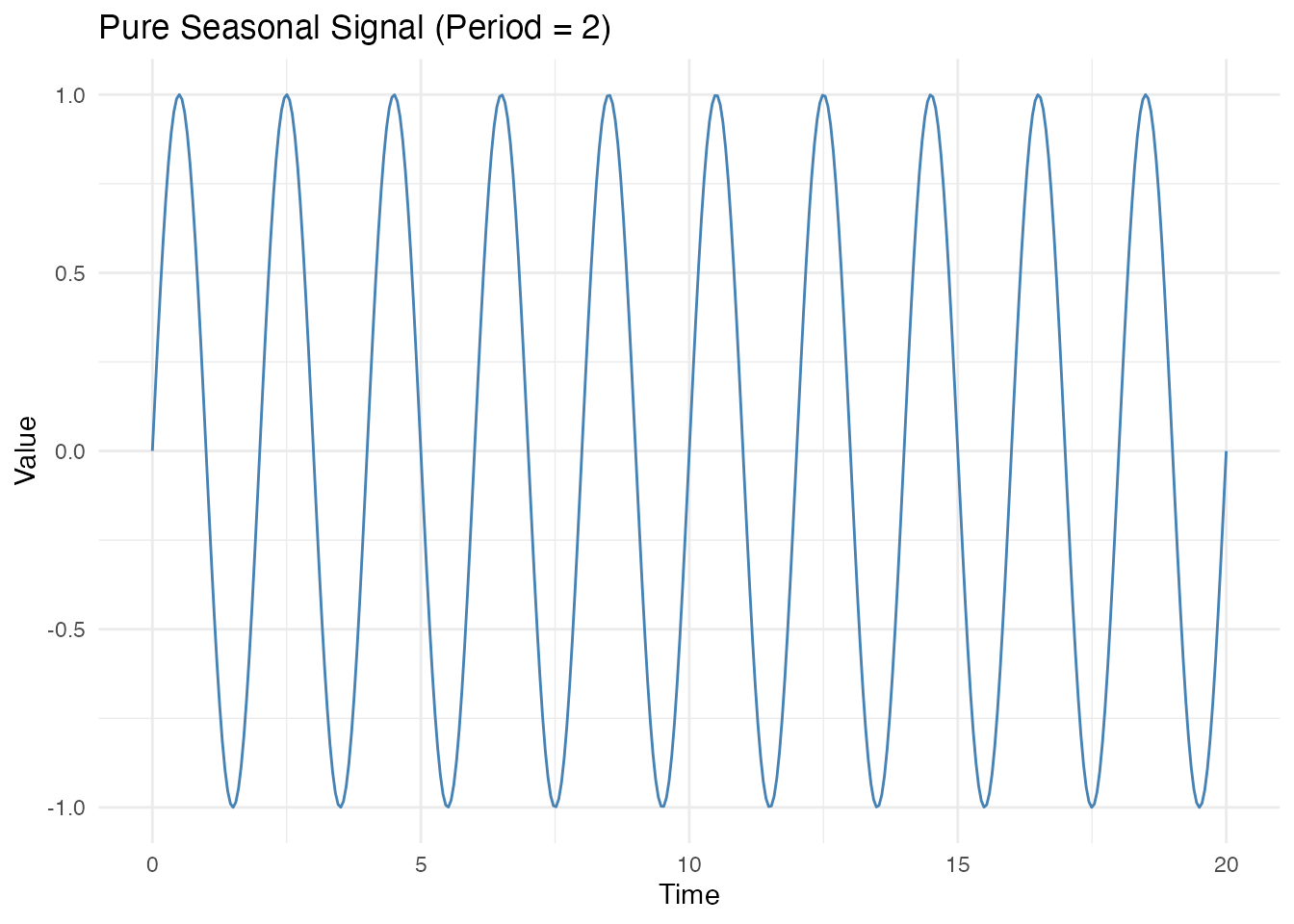

# FFT method
est_fft <- estimate.period(fd_pure, method = "fft")
cat("FFT estimate:", est_fft$period, "(true:", period_true, ")\n")
#> FFT estimate: 2.005013 (true: 2 )
cat("Confidence:", round(est_fft$confidence, 3), "\n")
#> Confidence: 199.585

The confidence value indicates how pronounced the dominant frequency is relative to other frequencies. High confidence (close to 1) means a clear, dominant period.

Noisy Signals

Real data always contains noise. Let’s see how the methods handle it.

# Add noise
X_noisy <- sin(2 * pi * t / period_true) + rnorm(length(t), sd = 0.3)
fd_noisy <- fdata(matrix(X_noisy, nrow = 1), argvals = t)

df <- data.frame(t = t, y = X_noisy)
ggplot(df, aes(x = t, y = y)) +
  geom_line(color = "steelblue", alpha = 0.7) +
  labs(title = "Noisy Seasonal Signal (SD = 0.3)", x = "Time", y = "Value")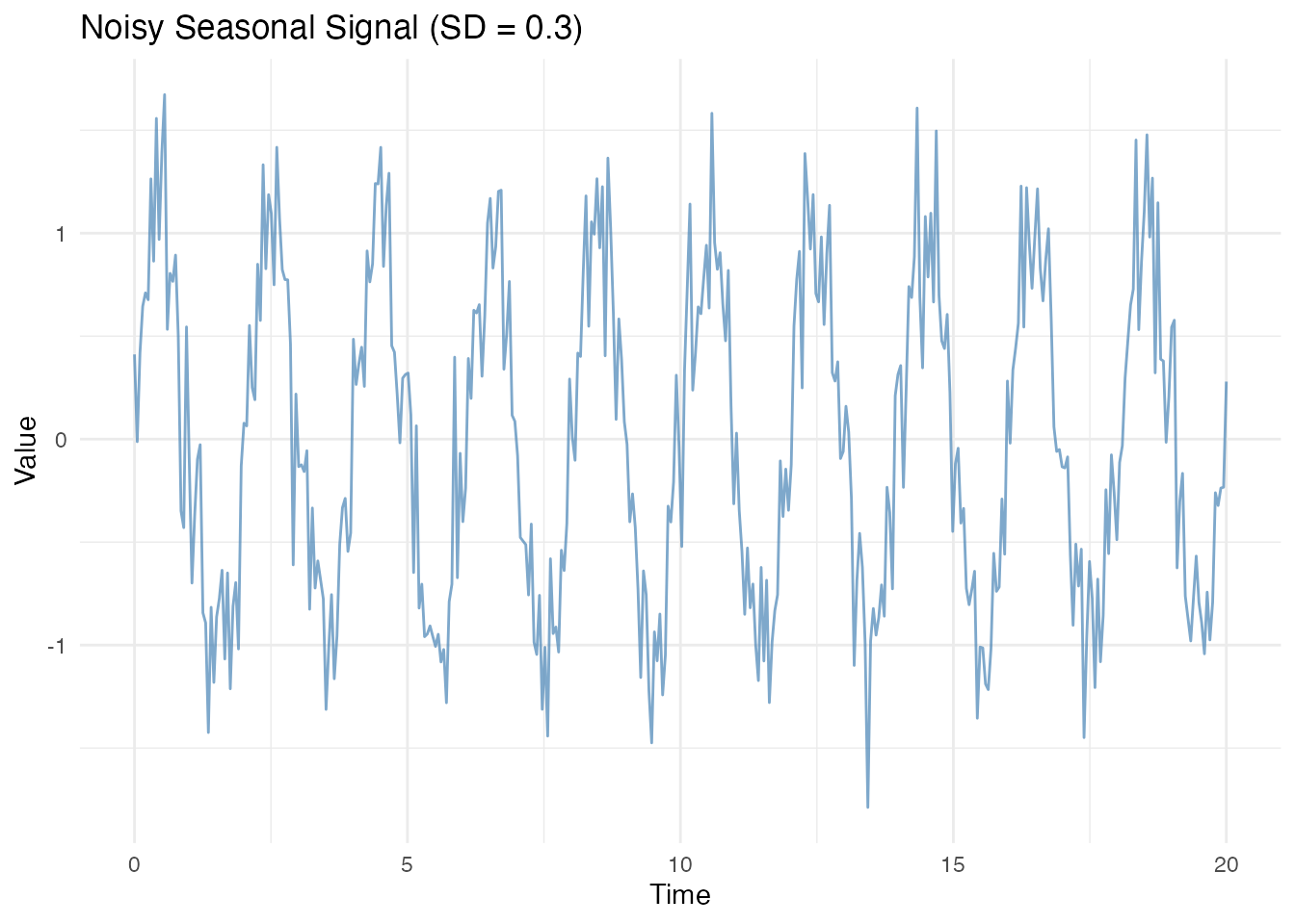

# Compare methods
est_fft_noisy <- estimate.period(fd_noisy, method = "fft")
est_acf <- estimate.period(fd_noisy, method = "acf")

cat("True period:", period_true, "\n")
#> True period: 2
cat("FFT estimate:", est_fft_noisy$period, "(confidence:", round(est_fft_noisy$confidence, 3), ")\n")
#> FFT estimate: 2.005013 (confidence: 171.93 )
cat("ACF estimate:", est_acf$period, "(confidence:", round(est_acf$confidence, 3), ")\n")
#> ACF estimate: 2.005013 (confidence: 0.783 )

Both methods typically agree for clean periodic signals. The ACF method can be more robust to certain types of noise, while FFT is faster and handles multiple harmonics well.

Signals with Multiple Harmonics

Real seasonal patterns often have harmonics (e.g., yearly + half-yearly components that share the same fundamental period).

# Signal with 2nd and 3rd harmonics
X_multi <- sin(2 * pi * t / period_true) +
           0.3 * sin(4 * pi * t / period_true) +  # 2nd harmonic
           0.1 * sin(6 * pi * t / period_true) +  # 3rd harmonic
           rnorm(length(t), sd = 0.1)
fd_multi <- fdata(matrix(X_multi, nrow = 1), argvals = t)

df <- data.frame(t = t, y = X_multi)
ggplot(df, aes(x = t, y = y)) +
  geom_line(color = "steelblue") +
  labs(title = "Signal with Multiple Harmonics", x = "Time", y = "Value")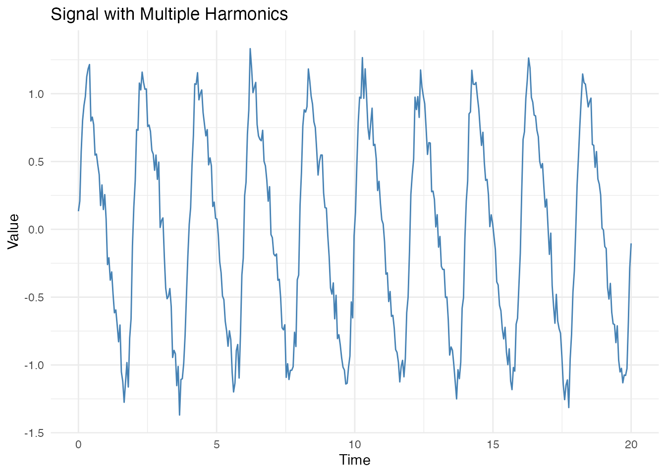

est_multi <- estimate.period(fd_multi, method = "fft")
cat("Estimated period:", est_multi$period, "(true:", period_true, ")\n")
#> Estimated period: 2.005013 (true: 2 )

The FFT method correctly identifies the fundamental period, even when harmonics are present. The harmonics share the same fundamental frequency, so they reinforce the estimate.

Detecting Multiple Concurrent Seasonalities

Sometimes a signal contains multiple independent periodicities (e.g., daily and yearly cycles). The estimate.period() function returns only the dominant period. Here’s how to detect multiple periods.

Why estimate.period() Returns Only One Period

# Signal with two independent periods
period1 <- 2   # Fast cycle
period2 <- 7   # Slow cycle

X_dual <- sin(2 * pi * t / period1) + 0.6 * sin(2 * pi * t / period2)
fd_dual <- fdata(matrix(X_dual, nrow = 1), argvals = t)

df <- data.frame(t = t, y = X_dual)
ggplot(df, aes(x = t, y = y)) +
  geom_line(color = "steelblue") +
  labs(title = "Signal with Two Periods (2 and 7)",
       x = "Time", y = "Value")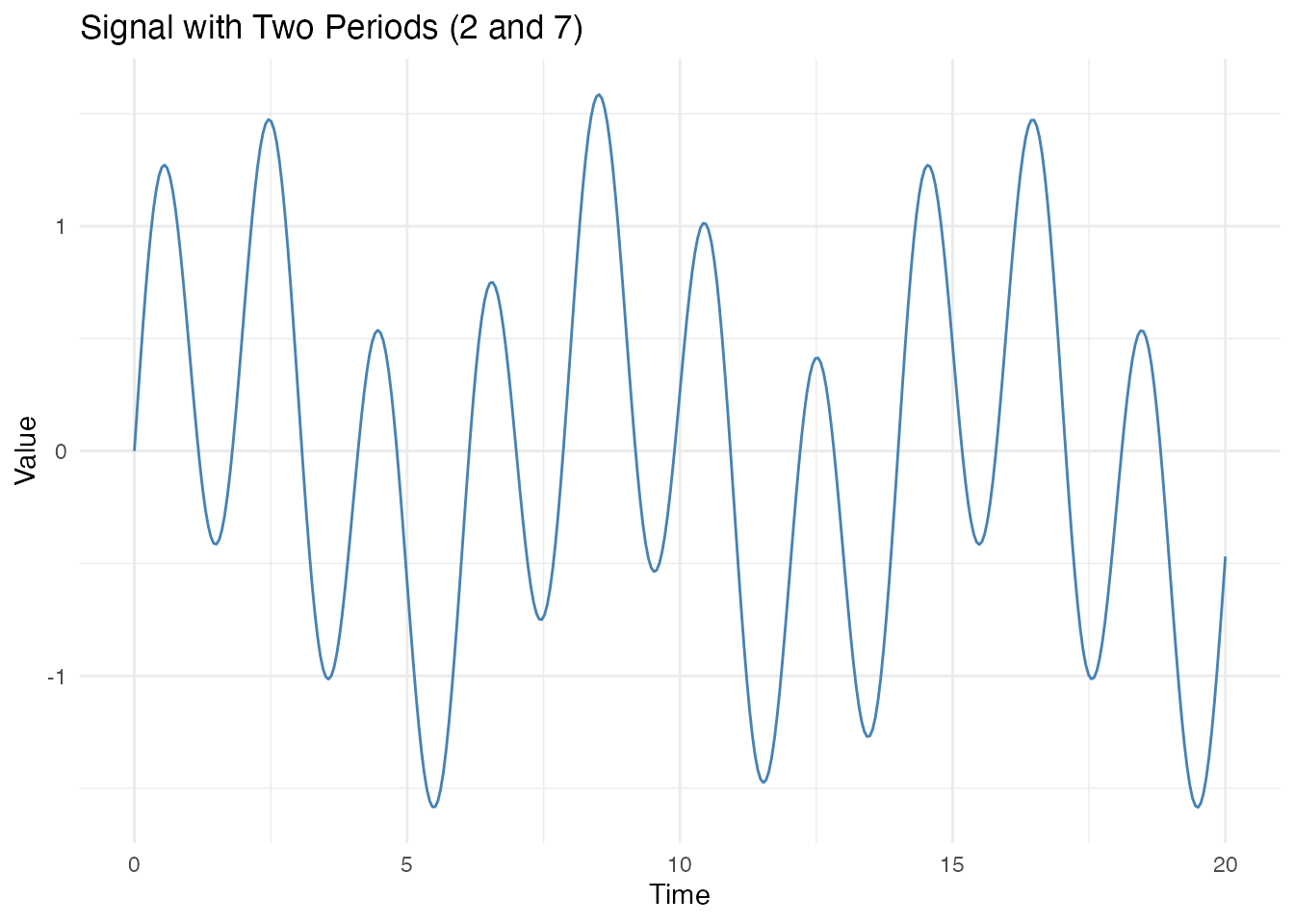

est_single <- estimate.period(fd_dual, method = "fft")
cat("Single estimate:", est_single$period, "\n")
#> Single estimate: 2.005013
cat("(Only detects the dominant period)\n")
#> (Only detects the dominant period)

Using detect.periods()

The detect.periods() function uses an iterative residual approach implemented in Rust for efficiency:

1. Estimate the dominant period using FFT
2. Subtract a fitted sinusoid at that period
3. Repeat on the residual until confidence or strength drops too low

# Detect multiple periods using the package function
# Higher thresholds prevent spurious detection
detected <- detect.periods(fd_dual, max_periods = 3,
                                     min_confidence = 0.5,
                                     min_strength = 0.25)
print(detected)
#> Multiple Period Detection
#> -------------------------
#> Periods detected: 3
#> 
#> Period 1: 2.005 (confidence=148.091, strength=0.741, amplitude=0.956)
#> Period 2: 6.683 (confidence=123.084, strength=0.628, amplitude=0.444)
#> Period 3: 10.025 (confidence=128.631, strength=0.705, amplitude=0.282)

Visualizing the Decomposition

# Reconstruct each component using detected periods
components <- data.frame(t = t)
residual <- X_dual

if (detected$n_periods > 0) {
  for (i in seq_len(detected$n_periods)) {
    omega <- 2 * pi / detected$periods[i]
    cos_comp <- cos(omega * t)
    sin_comp <- sin(omega * t)
    a <- 2 * mean(residual * cos_comp)
    b <- 2 * mean(residual * sin_comp)
    component <- a * cos_comp + b * sin_comp
    components[[paste0("Period_", round(detected$periods[i], 1))]] <- component
    residual <- residual - component
  }
}
components$Residual <- residual
components$Original <- X_dual

# Plot decomposition
library(tidyr)
df_long <- pivot_longer(components, -t, names_to = "Component", values_to = "Value")
# Get period column names (exclude t, Residual, Original)
period_cols <- setdiff(names(components), c("t", "Residual", "Original"))
df_long$Component <- factor(df_long$Component,
                            levels = c("Original", period_cols, "Residual"))

ggplot(df_long, aes(x = t, y = Value)) +
  geom_line(color = "steelblue") +
  facet_wrap(~Component, ncol = 1, scales = "free_y") +
  labs(title = "Decomposition into Periodic Components",
       x = "Time", y = "Value")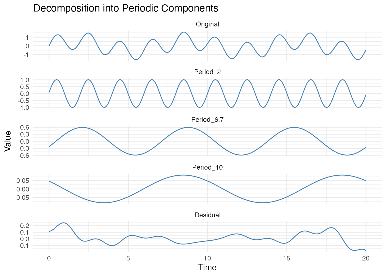

Practical guidance:

• For harmonics of the same fundamental: estimate.period() correctly finds the fundamental period. No iterative approach needed.
• For truly different periods (e.g., daily + yearly): use the iterative approach above.
• When confidence drops below threshold: stop - remaining signal is likely noise.

Note on detection order: Periods are detected in order of amplitude, not period length. The component with the highest FFT power (roughly proportional to amplitude squared) is found first. For example, if a signal has a weak yearly cycle and a strong weekly cycle, the weekly cycle will be detected first regardless of which period is longer. Very weak periodicities (< 20% of the dominant amplitude) may require lower thresholds but risk false positives.

Handling Non-Stationary Data

Real-world time series often have trends that can mask or distort seasonal patterns. fdars provides comprehensive detrending and decomposition functions to handle this.

The Problem: Trends Mask Seasonality

When a strong trend is present, seasonal analysis functions may fail:

# Signal with strong linear trend + seasonality + noise
t <- seq(0, 20, length.out = 400)
X_trend <- 5 + 2 * t + sin(2 * pi * t / 2.5) + rnorm(length(t), sd = 0.3)
fd_trend <- fdata(matrix(X_trend, nrow = 1), argvals = t)

df <- data.frame(t = t, y = X_trend)
ggplot(df, aes(x = t, y = y)) +
  geom_line(color = "steelblue") +
  labs(title = "Seasonal Signal with Strong Linear Trend",
       subtitle = "The trend dominates, masking the seasonality",
       x = "Time", y = "Value")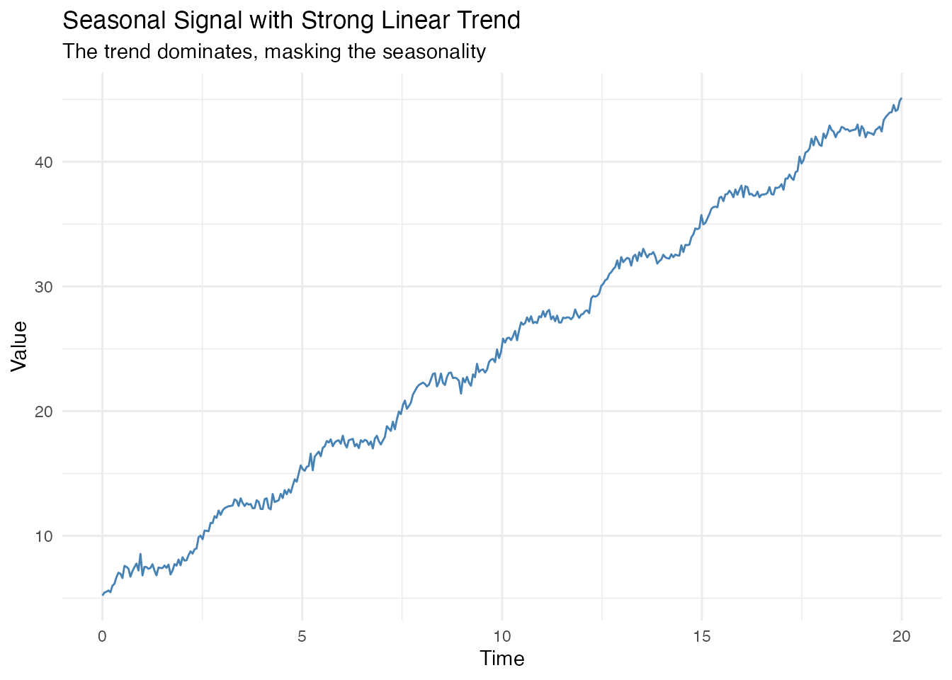

# Without detrending - incorrect results!
period_wrong <- estimate.period(fd_trend)$period
strength_wrong <- seasonal.strength(fd_trend, period = 2.5)

cat("WITHOUT detrending:\n")
#> WITHOUT detrending:
cat("  Estimated period:", round(period_wrong, 2), "(true: 2.5)\n")
#>   Estimated period: 20.05 (true: 2.5)
cat("  Seasonal strength:", round(strength_wrong, 3), "(should be ~1)\n")
#>   Seasonal strength: 0.005 (should be ~1)

The trend causes: - Period estimation to return the series length (20) instead of the true period (2.5) - Seasonal strength to be nearly zero, when it should be close to 1

Using detrend()

The detrend() function removes trends using various methods:

# Linear detrending
fd_linear <- detrend(fd_trend, method = "linear")

# Polynomial detrending (degree 2)
fd_poly <- detrend(fd_trend, method = "polynomial", degree = 2)

# LOESS detrending (flexible, non-parametric)
fd_loess <- detrend(fd_trend, method = "loess", bandwidth = 0.3)

# Automatic selection via AIC
fd_auto <- detrend(fd_trend, method = "auto")

# Compare results
cat("After detrending, estimated periods:\n")
#> After detrending, estimated periods:
cat("  Linear:     ", round(estimate.period(fd_linear)$period, 3), "\n")
#>   Linear:      2.506
cat("  Polynomial: ", round(estimate.period(fd_poly)$period, 3), "\n")
#>   Polynomial:  2.506
cat("  LOESS:      ", round(estimate.period(fd_loess)$period, 3), "\n")
#>   LOESS:       2.506
cat("  Auto:       ", round(estimate.period(fd_auto)$period, 3), "(true: 2.5)\n")
#>   Auto:        2.506 (true: 2.5)

Getting Both Trend and Detrended Data

Use return_trend = TRUE to get both components:

result <- detrend(fd_trend, method = "linear", return_trend = TRUE)

# Plot original, trend, and detrended
df_decomp <- data.frame(
  t = rep(t, 3),
  y = c(fd_trend$data[1,], result$trend$data[1,], result$detrended$data[1,]),
  Component = factor(rep(c("Original", "Trend", "Detrended"), each = length(t)),
                     levels = c("Original", "Trend", "Detrended"))
)

ggplot(df_decomp, aes(x = t, y = y)) +
  geom_line(color = "steelblue") +
  facet_wrap(~Component, ncol = 1, scales = "free_y") +
  labs(title = "Linear Detrending Result",
       x = "Time", y = "Value")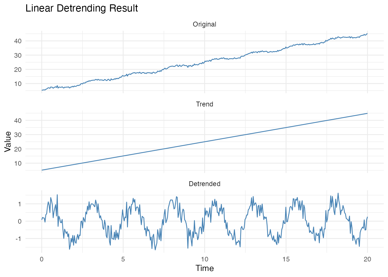

Seasonal-Trend Decomposition

For full decomposition into trend, seasonal, and remainder components, use decompose():

# Additive decomposition: data = trend + seasonal + remainder
decomp <- decompose(fd_trend, period = 2.5, method = "additive")

# Plot all components
df_stl <- data.frame(
  t = rep(t, 4),
  y = c(fd_trend$data[1,], decomp$trend$data[1,],
        decomp$seasonal$data[1,], decomp$remainder$data[1,]),
  Component = factor(rep(c("Original", "Trend", "Seasonal", "Remainder"), each = length(t)),
                     levels = c("Original", "Trend", "Seasonal", "Remainder"))
)

ggplot(df_stl, aes(x = t, y = y)) +
  geom_line(color = "steelblue") +
  facet_wrap(~Component, ncol = 1, scales = "free_y") +
  labs(title = "Additive Seasonal-Trend Decomposition",
       x = "Time", y = "Value")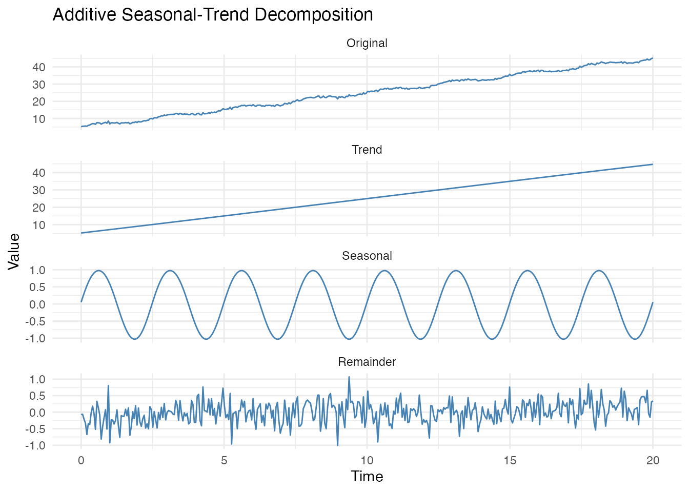

Multiplicative Seasonality

When the seasonal amplitude grows with the trend level, use multiplicative decomposition:

# Multiplicative pattern: amplitude grows with level + noise
X_mult <- (2 + 0.3 * t) * (1 + 0.4 * sin(2 * pi * t / 2.5)) + rnorm(length(t), sd = 0.5)
fd_mult <- fdata(matrix(X_mult, nrow = 1), argvals = t)

# Plot - note how peaks get taller over time
df_mult <- data.frame(t = t, y = X_mult)
ggplot(df_mult, aes(x = t, y = y)) +
  geom_line(color = "steelblue") +
  labs(title = "Multiplicative Seasonality",
       subtitle = "Seasonal amplitude grows with trend level",
       x = "Time", y = "Value")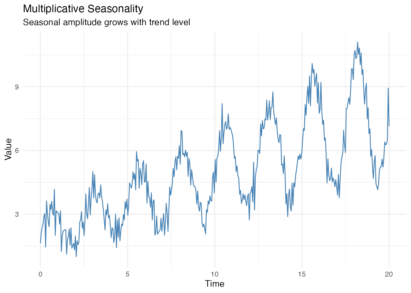

# Multiplicative decomposition
decomp_mult <- decompose(fd_mult, period = 2.5, method = "multiplicative")

cat("Multiplicative decomposition:\n")
#> Multiplicative decomposition:
cat("  Seasonal range:", round(range(decomp_mult$seasonal$data[1,]), 3), "\n")
#>   Seasonal range: 0.631 1.469
cat("  (Values near 1 indicate multiplicative factors)\n")
#>   (Values near 1 indicate multiplicative factors)

Integrated Detrending in Other Functions

All main seasonal functions support a detrend_method parameter:

# These are equivalent:
# 1. Explicit detrending
fd_det <- detrend(fd_trend, method = "linear")
p1 <- estimate.period(fd_det)$period

# 2. Integrated detrending parameter
p2 <- estimate.period(fd_trend, detrend_method = "linear")$period

cat("Explicit detrend:", round(p1, 3), "\n")
#> Explicit detrend: 2.506
cat("Integrated param:", round(p2, 3), "\n")
#> Integrated param: 2.506

The detrend_method parameter is available in: - estimate.period() - For accurate period estimation on trending data - detect.peaks() - For correct peak prominence calculation - seasonal.strength() - For true seasonality measurement - detect.periods() - Uses “auto” by default

# Dramatic improvement with detrending
cat("\nSeasonal strength comparison:\n")
#> 
#> Seasonal strength comparison:
cat("  Without detrend:", round(seasonal.strength(fd_trend, period = 2.5), 3), "\n")
#>   Without detrend: 0.005
cat("  With detrend:   ", round(seasonal.strength(fd_trend, period = 2.5,
                                                   detrend_method = "linear"), 3), "\n")
#>   With detrend:    0.834

Peak Detection with Detrending

Trends also affect peak detection - the upward slope can distort prominence calculations and make later peaks appear more prominent than earlier ones.

# Detect peaks without detrending
peaks_no_detrend <- detect.peaks(fd_trend, min_distance = 2, smooth_first = TRUE)

# Detect peaks with detrending
peaks_with_detrend <- detect.peaks(fd_trend, min_distance = 2, smooth_first = TRUE,
                                    detrend_method = "linear")

cat("Peak detection on trending data:\n")
#> Peak detection on trending data:
cat("  Without detrend:", nrow(peaks_no_detrend$peaks[[1]]), "peaks,",
    "mean period:", round(peaks_no_detrend$mean_period, 3), "\n")
#>   Without detrend: 5 peaks, mean period: 4.398
cat("  With detrend:   ", nrow(peaks_with_detrend$peaks[[1]]), "peaks,",
    "mean period:", round(peaks_with_detrend$mean_period, 3), "(true: 2.5)\n")
#>   With detrend:    8 peaks, mean period: 2.506 (true: 2.5)

# Visualize the difference
peaks_raw <- peaks_no_detrend$peaks[[1]]
peaks_det <- peaks_with_detrend$peaks[[1]]

# Get detrended data for plotting
fd_detrended <- detrend(fd_trend, method = "linear")

df_peaks <- data.frame(
  t = rep(t, 2),
  y = c(fd_trend$data[1,], fd_detrended$data[1,]),
  Panel = factor(rep(c("Original (with trend)", "Detrended"), each = length(t)),
                 levels = c("Original (with trend)", "Detrended"))
)

# Combine peak data
peaks_raw$Panel <- "Original (with trend)"
peaks_det$Panel <- "Detrended"
# Adjust detrended peak values to match detrended data
peaks_det$value <- fd_detrended$data[1, sapply(peaks_det$time, function(x) which.min(abs(t - x)))]
peaks_combined <- rbind(peaks_raw, peaks_det)
peaks_combined$Panel <- factor(peaks_combined$Panel,
                                levels = c("Original (with trend)", "Detrended"))

ggplot(df_peaks, aes(x = t, y = y)) +
  geom_line(color = "steelblue", alpha = 0.7) +
  geom_point(data = peaks_combined, aes(x = time, y = value),
             color = "red", size = 2) +
  facet_wrap(~Panel, ncol = 1, scales = "free_y") +
  labs(title = "Peak Detection: With vs Without Detrending",
       subtitle = "Detrending ensures consistent peak detection across the series",
       x = "Time", y = "Value")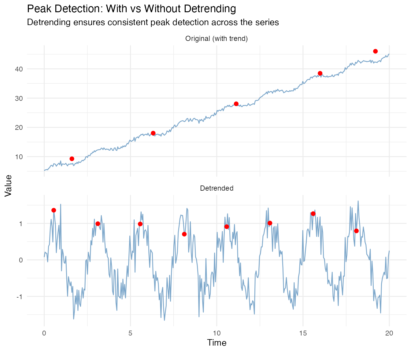

Detrending is especially important when: - Peaks near the start/end of the series have different prominence due to the trend - You need consistent peak-to-peak period estimates - The trend slope is comparable to or larger than the seasonal amplitude

Choosing a Detrending Method

Method	Use When	Parameters
"linear"	Simple linear trends	None
"polynomial"	Curved trends (quadratic, cubic)	degree (2, 3, etc.)
"loess"	Complex, irregular trends	bandwidth (0.1-0.5)
"diff1"	Random walk-like data	None (reduces length by 1)
"diff2"	Integrated processes	None (reduces length by 2)
"auto"	Unknown trend type	Selects via AIC

Recommendation: Start with "linear" for most cases. Use "auto" if unsure. Use "loess" for complex trends that polynomial methods cannot capture.

Peak Detection

Peak detection identifies local maxima in seasonal signals. This is useful for characterizing seasonal patterns and estimating period from peak-to-peak distances.

Parameter Tuning Guide

Peak detection quality depends heavily on parameters. Here’s a reference:

Parameter	Purpose	Typical Values	When to Adjust
min_distance	Minimum time between peaks	period * 0.8	Set to ~80% of expected period
min_prominence	How much peak stands out	0.1-0.5 x amplitude	Increase if too many noise peaks
smooth_first	Pre-smooth noisy data	TRUE for real data	Almost always use TRUE
smooth_nbasis	Number of Fourier basis	NULL (auto CV)	Let CV choose optimal nbasis

Effect of Parameters

Let’s demonstrate how parameters affect detection quality.

# Moderately noisy signal
X_demo <- sin(2 * pi * t / period_true) + rnorm(length(t), sd = 0.4)
fd_demo <- fdata(matrix(X_demo, nrow = 1), argvals = t)

df <- data.frame(t = t, y = X_demo)

Visualizing the Smoothing Step

Before detecting peaks, let’s see what Fourier basis smoothing does to noisy data:

# Apply Fourier basis smoothing with CV-selected optimal nbasis
cv_result <- fdata2basis_cv(fd_demo, nbasis.range = 5:25, type = "fourier", criterion = "GCV")
fd_smoothed <- cv_result$fitted

# Compare original vs smoothed
df_smooth <- data.frame(
  t = rep(t, 2),
  y = c(X_demo, fd_smoothed$data[1, ]),
  type = rep(c("Original (noisy)", "Smoothed (Fourier)"), each = length(t))
)

ggplot(df_smooth, aes(x = t, y = y, color = type)) +
  geom_line(linewidth = 0.8) +
  scale_color_manual(values = c("Original (noisy)" = "gray50",
                                 "Smoothed (Fourier)" = "steelblue")) +
  labs(title = "Effect of Fourier Basis Smoothing on Noisy Signal",
       subtitle = paste("CV-selected optimal nbasis =", cv_result$optimal.nbasis),
       x = "Time", y = "Value", color = NULL) +
  theme(legend.position = "bottom")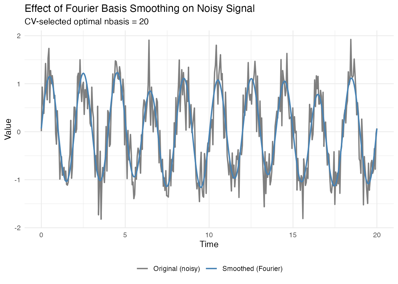

Fourier basis smoothing is ideal for seasonal signals because it naturally captures periodic patterns. Peak detection on the smoothed data will find the true peaks, not noise spikes.

# Default parameters - often too many peaks
peaks_default <- detect.peaks(fd_demo)
cat("Default parameters:", nrow(peaks_default$peaks[[1]]), "peaks found\n")
#> Default parameters: 96 peaks found
cat("(Expected:", floor(max(t) / period_true), "peaks)\n")
#> (Expected: 10 peaks)

# Add minimum distance constraint
peaks_distance <- detect.peaks(fd_demo, min_distance = period_true * 0.8)
cat("With min_distance:", nrow(peaks_distance$peaks[[1]]), "peaks found\n")
#> With min_distance: 12 peaks found

# Add Fourier smoothing for best results (GCV auto-selects nbasis)
peaks_smooth <- detect.peaks(fd_demo, min_distance = period_true * 0.8,
                             smooth_first = TRUE, smooth_nbasis = NULL)
cat("With smoothing:", nrow(peaks_smooth$peaks[[1]]), "peaks found\n")
#> With smoothing: 10 peaks found
cat("Estimated period from peaks:", round(peaks_smooth$mean_period, 3), "\n")
#> Estimated period from peaks: 1.999

Visualizing the Difference

# Prepare data for plotting
df_default <- peaks_default$peaks[[1]]
df_distance <- peaks_distance$peaks[[1]]
df_smooth <- peaks_smooth$peaks[[1]]

# Create combined plot
p1 <- ggplot(df, aes(x = t, y = y)) +
  geom_line(color = "gray50", alpha = 0.7) +
  geom_point(data = df_default, aes(x = time, y = value),
             color = "red", size = 2) +
  labs(title = paste("Default:", nrow(df_default), "peaks"),
       x = "", y = "Value")

p2 <- ggplot(df, aes(x = t, y = y)) +
  geom_line(color = "gray50", alpha = 0.7) +
  geom_point(data = df_distance, aes(x = time, y = value),
             color = "red", size = 2) +
  labs(title = paste("With min_distance:", nrow(df_distance), "peaks"),
       x = "", y = "Value")

p3 <- ggplot(df, aes(x = t, y = y)) +
  geom_line(color = "gray50", alpha = 0.7) +
  geom_point(data = df_smooth, aes(x = time, y = value),
             color = "red", size = 2) +
  labs(title = paste("With smoothing:", nrow(df_smooth), "peaks"),
       x = "Time", y = "Value")

library(gridExtra)
grid.arrange(p1, p2, p3, ncol = 1)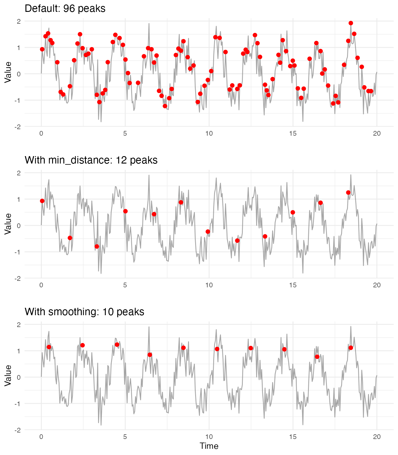

Why peak detection in noisy signals is challenging: Noise creates many local maxima that are not true peaks. Without smoothing, peak detection algorithms struggle to distinguish genuine seasonal peaks from random fluctuations. The min_distance parameter helps, but cannot fully solve the problem when noise amplitude is comparable to the signal.

Key insight: For seasonal data, use Fourier basis smoothing with smooth_first = TRUE. The Fourier basis is ideal for periodic signals because it naturally captures oscillatory patterns while suppressing noise. GCV automatically selects the optimal number of basis functions, balancing smoothness and fidelity to the data.

Prominence Filtering

Prominence measures how much a peak stands out from surrounding values. Use it to filter minor peaks. For best results with noisy data, combine prominence filtering with smoothing.

# Compare prominence thresholds without smoothing (less reliable)
peaks_low_prom_raw <- detect.peaks(fd_demo, min_distance = 1.5, min_prominence = 0.1)
peaks_high_prom_raw <- detect.peaks(fd_demo, min_distance = 1.5, min_prominence = 0.5)

cat("Without smoothing:\n")
#> Without smoothing:
cat("  Low prominence (0.1):", nrow(peaks_low_prom_raw$peaks[[1]]), "peaks\n")
#>   Low prominence (0.1): 7 peaks
cat("  High prominence (0.5):", nrow(peaks_high_prom_raw$peaks[[1]]), "peaks\n")
#>   High prominence (0.5): 1 peaks

# With smoothing - more reliable results
peaks_low_prom <- detect.peaks(fd_demo, min_distance = 1.5, min_prominence = 0.1,
                                smooth_first = TRUE)
peaks_high_prom <- detect.peaks(fd_demo, min_distance = 1.5, min_prominence = 0.5,
                                 smooth_first = TRUE)

cat("\nWith smoothing:\n")
#> 
#> With smoothing:
cat("  Low prominence (0.1):", nrow(peaks_low_prom$peaks[[1]]), "peaks\n")
#>   Low prominence (0.1): 4 peaks
cat("  High prominence (0.5):", nrow(peaks_high_prom$peaks[[1]]), "peaks\n")
#>   High prominence (0.5): 4 peaks

When smoothing is applied first, the prominence values become more meaningful because they reflect actual signal characteristics rather than noise artifacts.

Different Signal Amplitudes

Peak detection works correctly regardless of signal amplitude. The algorithm normalizes internally based on local signal characteristics.

t <- seq(0, 10, length.out = 200)
amplitudes <- c(0.5, 1.0, 2.0, 5.0)

# Create plots for each amplitude
amplitude_plots <- lapply(amplitudes, function(amp) {
  X <- matrix(amp * sin(2 * pi * t / 2), nrow = 1)
  fd <- fdata(X, argvals = t)
  result <- detect.peaks(fd)
  peaks <- result$peaks[[1]]

  df <- data.frame(t = t, y = X[1,])
  ggplot(df, aes(x = t, y = y)) +
    geom_line(color = "steelblue") +
    geom_point(data = peaks, aes(x = time, y = value),
               color = "red", size = 3) +
    labs(title = paste("Amplitude =", amp, "- Found", nrow(peaks), "peaks"),
         x = "Time", y = "Value")
})

library(gridExtra)
grid.arrange(grobs = amplitude_plots, ncol = 2)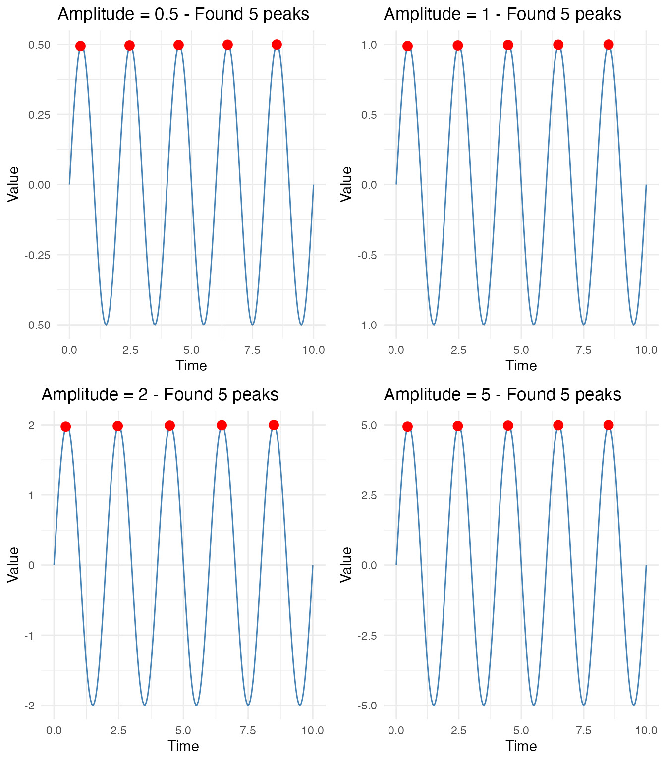

All four signals correctly detect 5 peaks, with peak values matching their respective amplitudes.

Non-Uniform Peak Spacing

Real-world signals often have varying frequencies or complex interference patterns. detect.peaks handles these cases by analyzing local signal structure.

Chirp Signal (Increasing Frequency)

A chirp signal has frequency that increases over time, causing peaks to get progressively closer together.

t <- seq(0, 10, length.out = 400)
# Phase integral for linearly increasing frequency: phi(t) = 2*pi*(0.5*t + 0.05*t^2)
phase <- 2 * pi * (0.5 * t + 0.05 * t^2)
X <- matrix(sin(phase), nrow = 1)
fd <- fdata(X, argvals = t)

result <- detect.peaks(fd)
peaks <- result$peaks[[1]]

# Plot
df <- data.frame(t = t, y = X[1,])
ggplot(df, aes(x = t, y = y)) +
  geom_line(color = "steelblue") +
  geom_point(data = peaks, aes(x = time, y = value),
             color = "red", size = 3) +
  labs(title = "Chirp Signal: Frequency Increases Over Time",
       subtitle = paste("Detected", nrow(peaks), "peaks with decreasing spacing"),
       x = "Time", y = "Value")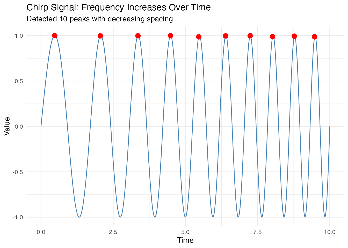

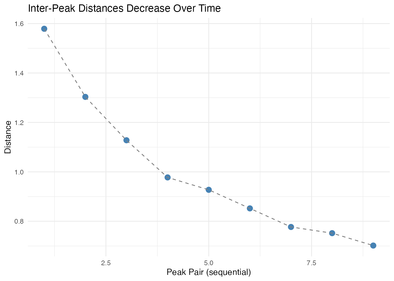
# Show inter-peak distances decreasing over time
distances <- result$inter_peak_distances[[1]]
if (length(distances) >= 2) {
  df_dist <- data.frame(
    peak_pair = seq_along(distances),
    distance = distances
  )
  ggplot(df_dist, aes(x = peak_pair, y = distance)) +
    geom_point(size = 3, color = "steelblue") +
    geom_line(linetype = "dashed", color = "gray50") +
    labs(title = "Inter-Peak Distances Decrease Over Time",
         x = "Peak Pair (sequential)", y = "Distance")
}

Sum of Sine Waves (Interference Pattern)

When two sine waves with different periods are combined, they create an interference pattern with non-uniform peak spacing.

t <- seq(0, 12, length.out = 300)
# Sum of periods 2 and 3
X <- matrix(sin(2 * pi * t / 2) + 0.5 * sin(2 * pi * t / 3), nrow = 1)
fd <- fdata(X, argvals = t)

result <- detect.peaks(fd, min_distance = 1.0)
peaks <- result$peaks[[1]]

# Plot
df <- data.frame(t = t, y = X[1,])
ggplot(df, aes(x = t, y = y)) +
  geom_line(color = "steelblue") +
  geom_point(data = peaks, aes(x = time, y = value),
             color = "red", size = 3) +
  labs(title = "Sum of Two Sine Waves (periods 2 and 3)",
       subtitle = paste("Detected", nrow(peaks), "peaks with varying spacing"),
       x = "Time", y = "Value")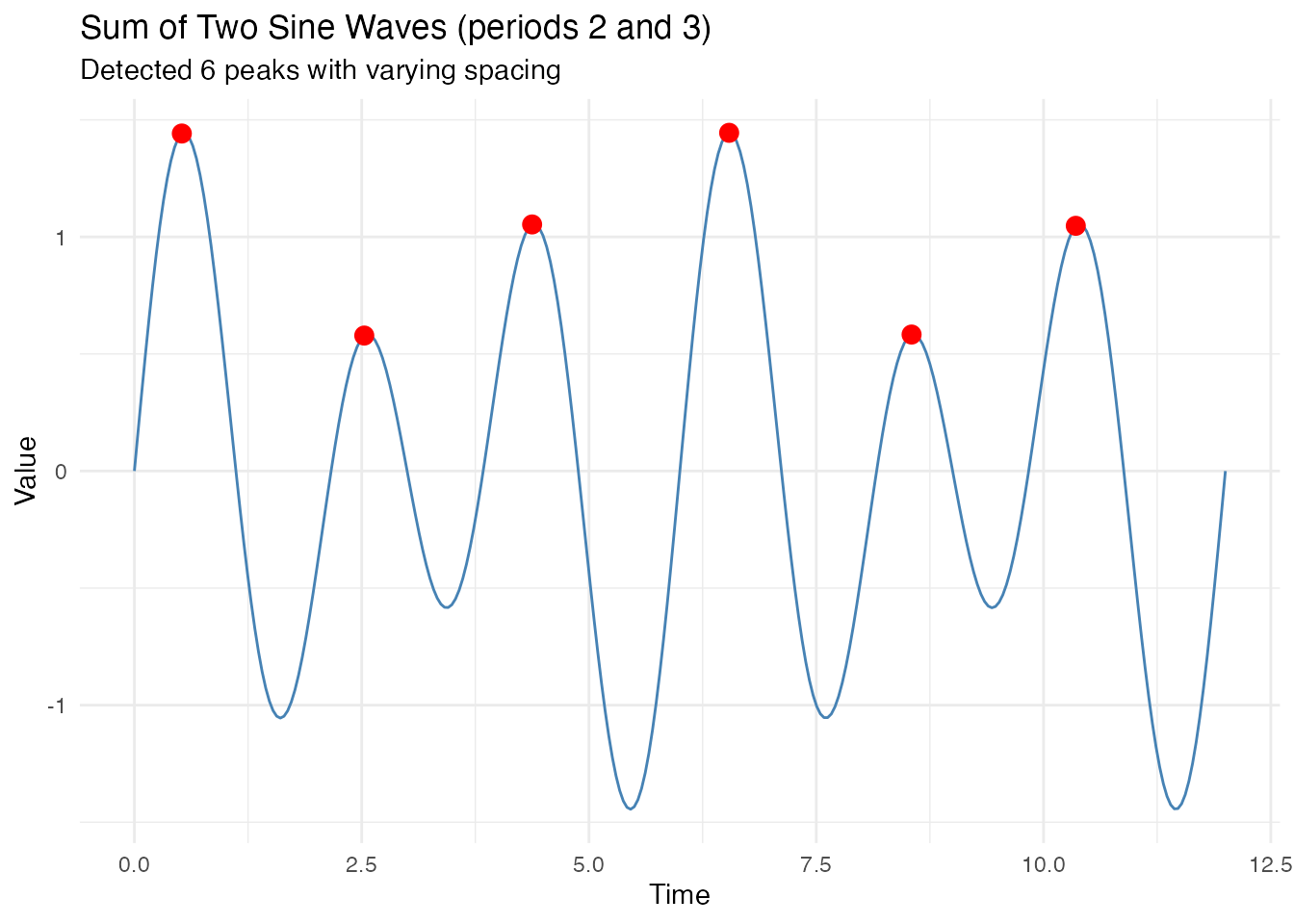

# Show variable inter-peak distances
distances <- result$inter_peak_distances[[1]]
cat("Inter-peak distances:", round(distances, 2), "\n")
#> Inter-peak distances: 2.01 1.85 2.17 2.01 1.81
cat("Range:", round(min(distances), 2), "to", round(max(distances), 2), "\n")
#> Range: 1.81 to 2.17

The peak detection algorithm correctly identifies local maxima even when the underlying signal has complex structure with varying peak-to-peak distances.

Measuring Seasonal Strength

Seasonal strength quantifies how much of the signal’s variance is explained by the seasonal component. Values range from 0 (no seasonality) to 1 (pure seasonal signal).

Variance vs Spectral Methods

ss_variance <- seasonal.strength(fd_noisy, period = period_true, method = "variance")
ss_spectral <- seasonal.strength(fd_noisy, period = period_true, method = "spectral")

cat("Variance method:", round(ss_variance, 3), "\n")
#> Variance method: 0.863
cat("Spectral method:", round(ss_spectral, 3), "\n")
#> Spectral method: 0.893

Comparing Different Signal Types

# Create signals with different seasonality levels
X_noise <- rnorm(length(t))  # Pure noise
fd_noise <- fdata(matrix(X_noise, nrow = 1), argvals = t)

X_mixed <- 0.5 * sin(2 * pi * t / period_true) + 0.5 * rnorm(length(t))
fd_mixed <- fdata(matrix(X_mixed, nrow = 1), argvals = t)

# Calculate strengths
strengths <- c(
  "Pure seasonal" = seasonal.strength(fd_pure, period = period_true),
  "Noisy seasonal (0.3 SD)" = seasonal.strength(fd_noisy, period = period_true),
  "Mixed (50/50)" = seasonal.strength(fd_mixed, period = period_true),
  "Pure noise" = seasonal.strength(fd_noise, period = period_true)
)

df_strength <- data.frame(
  Signal = factor(names(strengths), levels = names(strengths)),
  Strength = strengths
)

ggplot(df_strength, aes(x = Signal, y = Strength, fill = Signal)) +
  geom_col() +
  labs(title = "Seasonal Strength Comparison",
       x = "", y = "Seasonal Strength") +
  ylim(0, 1) +
  theme(legend.position = "none",
        axis.text.x = element_text(angle = 15, hjust = 1))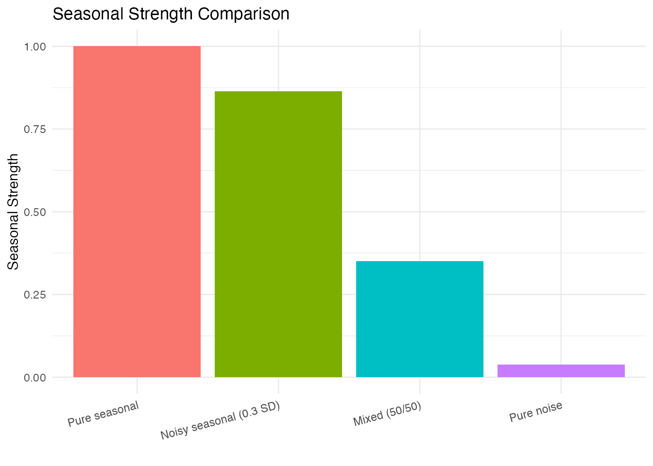

Time-Varying Seasonal Strength

Seasonal strength can change over time. Use a sliding window to track this.

# Signal that loses seasonality
t_long <- seq(0, 40, length.out = 800)
X_changing <- ifelse(t_long < 20,
                     sin(2 * pi * t_long / period_true) + rnorm(sum(t_long < 20), sd = 0.2),
                     rnorm(sum(t_long >= 20), sd = 0.5))
fd_changing <- fdata(matrix(X_changing, nrow = 1), argvals = t_long)

# Compute time-varying strength
ss_curve <- seasonal.strength.curve(fd_changing, period = period_true,
                                     window_size = 4 * period_true)

# Plot both signal and strength
df1 <- data.frame(t = t_long, y = X_changing, panel = "Signal")
df2 <- data.frame(t = t_long, y = ss_curve$data[1,], panel = "Seasonal Strength")
df_combined <- rbind(df1, df2)

ggplot(df_combined, aes(x = t, y = y)) +
  geom_line(color = "steelblue") +
  facet_wrap(~panel, ncol = 1, scales = "free_y") +
  geom_vline(xintercept = 20, linetype = "dashed", color = "red") +
  labs(title = "Time-Varying Seasonal Strength",
       subtitle = "Seasonality stops at t = 20 (red line)",
       x = "Time", y = "")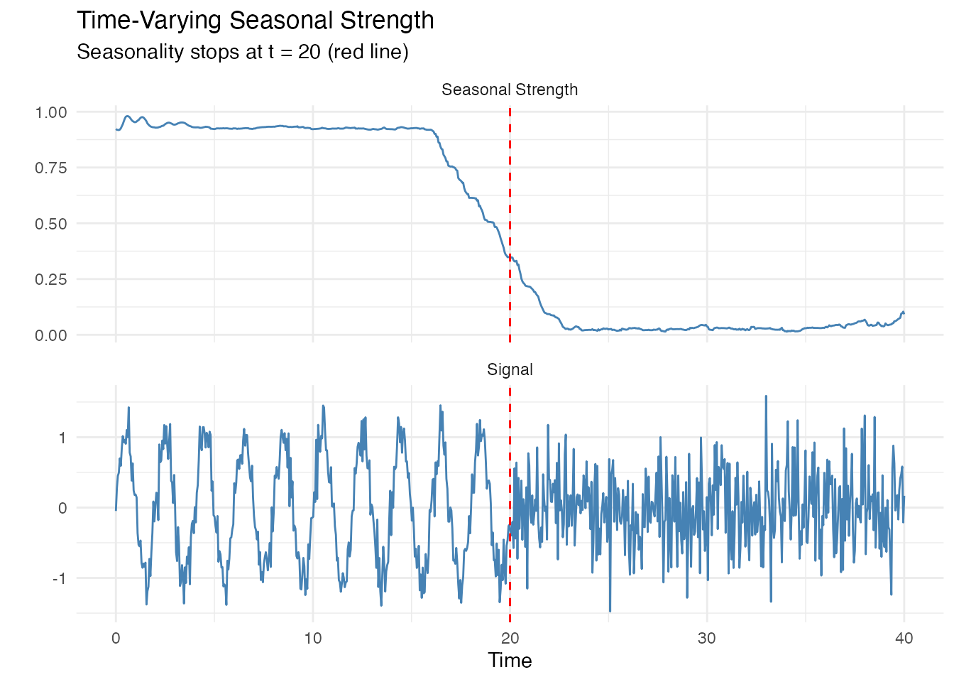

Change Detection

Automatically detect when seasonality starts or stops.

Manual Threshold

changes <- detect.seasonality.changes(fd_changing, period = period_true,
                                       threshold = 0.3,
                                       window_size = 4 * period_true,
                                       min_duration = 2 * period_true)
print(changes)
#> Seasonality Change Detection
#> ----------------------------
#> Number of changes: 1
#> 
#>       time      type strength_before strength_after
#> 1 20.47559 cessation       0.3152373      0.2918658

Automatic Threshold (Otsu’s Method)

When you don’t know the appropriate threshold, use Otsu’s method to determine it automatically from the data.

changes_auto <- detect.seasonality.changes.auto(fd_changing, period = period_true,
                                                 threshold_method = "otsu")
print(changes_auto)
#> Seasonality Change Detection (Auto Threshold)
#> ----------------------------------------------
#> Computed threshold: 0.5047
#> Number of changes: 1
#> 
#>       time      type strength_before strength_after
#> 1 19.52441 cessation       0.5087545      0.5030707

Visualizing Change Points

df <- data.frame(t = t_long, y = X_changing)

p <- ggplot(df, aes(x = t, y = y)) +
  geom_line(color = "steelblue", alpha = 0.7) +
  labs(title = "Seasonality Change Detection",
       x = "Time", y = "Value")

# Add change points
if (nrow(changes_auto$change_points) > 0) {
  for (i in 1:nrow(changes_auto$change_points)) {
    cp <- changes_auto$change_points[i, ]
    p <- p + geom_vline(xintercept = cp$time,
                        linetype = "dashed",
                        color = ifelse(cp$type == "onset", "green4", "red"),
                        linewidth = 1)
  }
  p <- p + labs(subtitle = "Green = onset, Red = cessation")
}
print(p)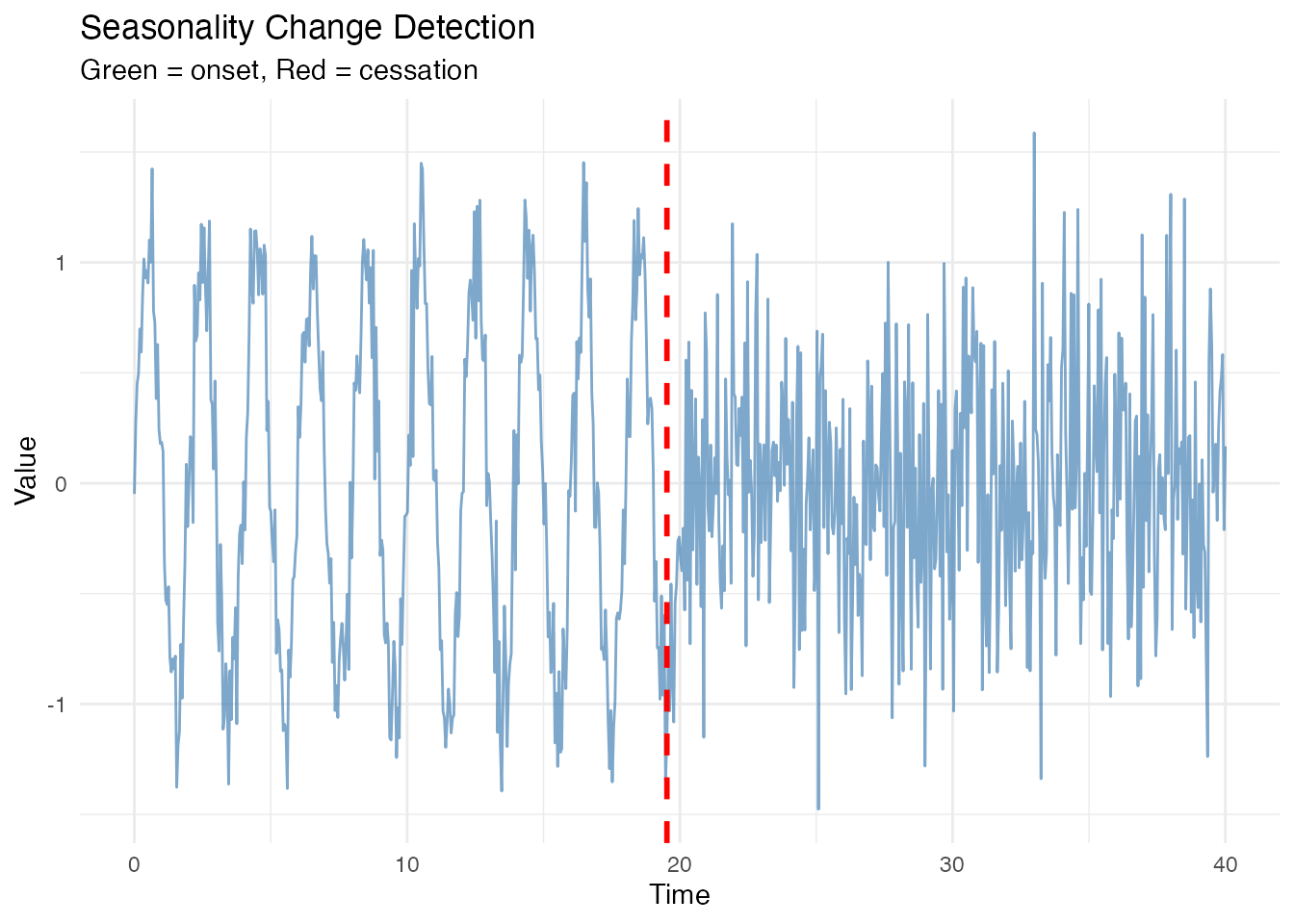

Signals with Varying Period

Some signals have periods that drift or change over time. The instantaneous.period() function uses the Hilbert transform to estimate the period at each time point.

When to Use Instantaneous Period

Good use cases:

• Slowly drifting systems (circadian rhythms shifting with seasons)
• Frequency-modulated (FM) signals in engineering
• Climate oscillations with variable period (e.g., ENSO)

Poor use cases:

• Random frequency jumps (use change detection instead)
• Multiple concurrent periodicities (use iterative approach instead)
• Very noisy short series (use peak-to-peak methods instead)

Chirp Signal (Smoothly Increasing Frequency)

# Chirp: frequency increases linearly
t_chirp <- seq(0, 10, length.out = 500)
freq <- 0.5 + 0.15 * t_chirp  # Frequency increases from 0.5 to 2
phase <- 2 * pi * cumsum(freq) * diff(c(0, t_chirp))
X_chirp <- sin(phase)
fd_chirp <- fdata(matrix(X_chirp, nrow = 1), argvals = t_chirp)

df <- data.frame(t = t_chirp, y = X_chirp)
ggplot(df, aes(x = t, y = y)) +
  geom_line(color = "steelblue") +
  labs(title = "Chirp Signal (Smoothly Increasing Frequency)",
       x = "Time", y = "Value")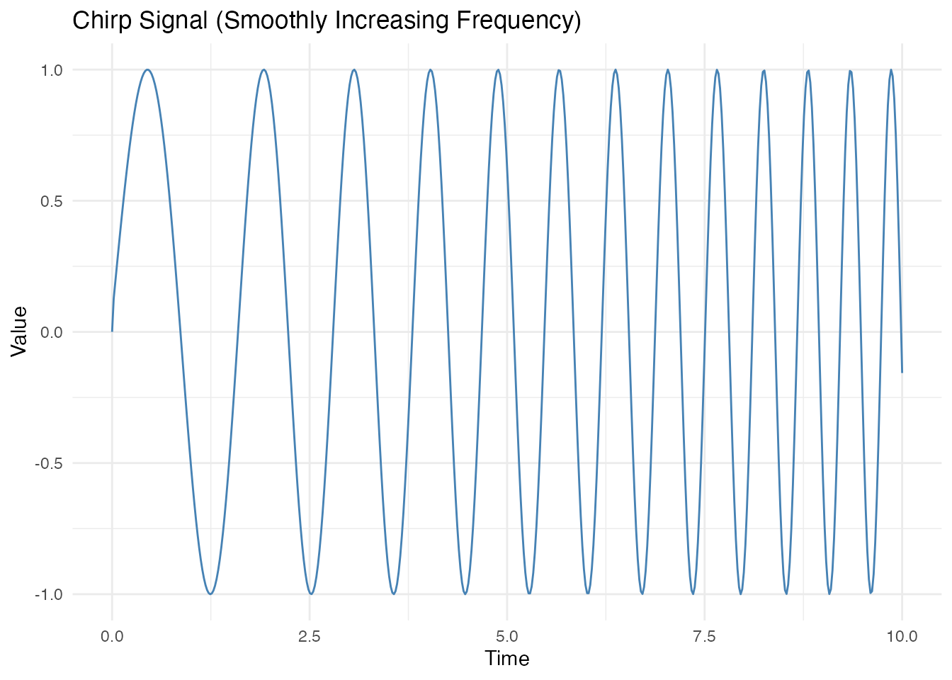

inst <- instantaneous.period(fd_chirp)

# True period (1/frequency)
true_period <- 1 / freq

# Compare
df <- data.frame(
  t = t_chirp,
  Estimated = inst$period$data[1,],
  True = true_period
)

# Remove extreme values at boundaries
df$Estimated[df$Estimated > 5 | df$Estimated < 0] <- NA

ggplot(df, aes(x = t)) +
  geom_line(aes(y = True, color = "True"), linewidth = 1) +
  geom_line(aes(y = Estimated, color = "Estimated"), alpha = 0.7) +
  scale_color_manual(values = c("True" = "steelblue", "Estimated" = "coral")) +
  labs(title = "Instantaneous Period Estimation",
       x = "Time", y = "Period", color = "") +
  ylim(0, 3)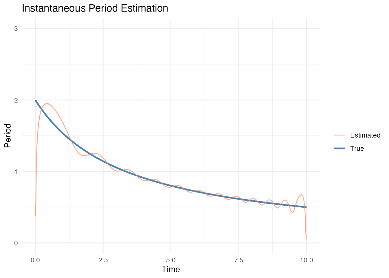

Amplitude Envelope Extraction

The Hilbert transform also provides the instantaneous amplitude (envelope), useful for amplitude-modulated signals.

# Amplitude-modulated signal
envelope_true <- 1 + 0.5 * sin(2 * pi * t / 10)  # Slow modulation
X_am <- envelope_true * sin(2 * pi * t / period_true)
fd_am <- fdata(matrix(X_am, nrow = 1), argvals = t)

inst_am <- instantaneous.period(fd_am)

df <- data.frame(
  t = t,
  Signal = X_am,
  Envelope = inst_am$amplitude$data[1,]
)

ggplot(df, aes(x = t)) +
  geom_line(aes(y = Signal), color = "steelblue", alpha = 0.7) +
  geom_line(aes(y = Envelope), color = "red", linewidth = 1) +
  geom_line(aes(y = -Envelope), color = "red", linewidth = 1) +
  labs(title = "Amplitude Envelope Extraction",
       subtitle = "Red lines show the extracted envelope",
       x = "Time", y = "Value")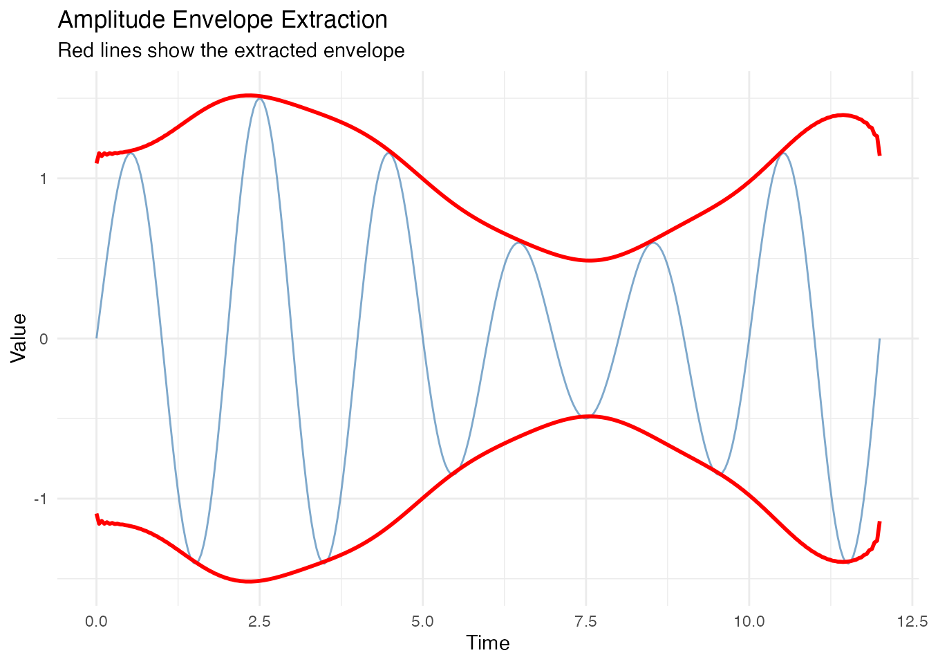

Limitations and Alternatives

Boundary effects: The Hilbert transform produces unreliable estimates near the beginning and end of the series.

Noise sensitivity: High-frequency noise can corrupt period estimates. Consider smoothing first.

Random frequency changes: When frequency changes abruptly and randomly, the instantaneous period estimate becomes unreliable.

# Demonstrate limitation: signal with random frequency regime changes
set.seed(123)
t_rand <- seq(0, 20, length.out = 400)
freq_regime <- rep(c(1, 2, 0.5, 1.5), each = 100)  # Abrupt changes
X_rand <- sin(2 * pi * cumsum(freq_regime) * diff(c(0, t_rand)))
fd_rand <- fdata(matrix(X_rand, nrow = 1), argvals = t_rand)

inst_rand <- instantaneous.period(fd_rand)
est_period <- inst_rand$period$data[1,]
est_period[est_period > 5 | est_period < 0.1] <- NA

df <- data.frame(
  t = t_rand,
  True = 1/freq_regime,
  Estimated = est_period
)

ggplot(df, aes(x = t)) +
  geom_step(aes(y = True, color = "True"), linewidth = 1) +
  geom_line(aes(y = Estimated, color = "Estimated"), alpha = 0.7) +
  scale_color_manual(values = c("True" = "steelblue", "Estimated" = "coral")) +
  labs(title = "Limitation: Abrupt Frequency Changes",
       subtitle = "Hilbert transform struggles with discontinuities",
       x = "Time", y = "Period", color = "")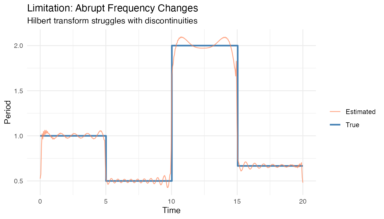

Alternative for abrupt changes: Use detect.seasonality.changes() to find regime boundaries, then analyze each segment separately.

Working with Short Series

For short series with only 3-5 complete cycles, fdars provides specialized functions for analyzing peak timing variability and classifying seasonality.

Challenges with Few Cycles

• Period estimation has limited frequency resolution
• Statistical measures have high uncertainty
• Peak-to-peak analysis becomes more important

Peak Timing Variability

Detect shifts in peak timing between cycles (e.g., a phenological event shifting from March to April to May over several years).

# Simulate 5 years where peak timing shifts
t_short <- seq(0, 5, length.out = 500)
period_short <- 1

# Peaks shift gradually later each year
phase_shifts <- c(0, 0.05, 0.10, 0.08, 0.04)
X_short <- rep(0, length(t_short))
for (i in 1:length(t_short)) {
  year <- floor(t_short[i]) + 1
  year <- min(year, 5)
  X_short[i] <- sin(2 * pi * (t_short[i] + phase_shifts[year]) / period_short)
}
X_short <- X_short + rnorm(length(t_short), sd = 0.1)

fd_short <- fdata(matrix(X_short, nrow = 1), argvals = t_short)

# Plot the short series
df_short <- data.frame(t = t_short, y = X_short)
ggplot(df_short, aes(x = t, y = y)) +
  geom_line(color = "steelblue") +
  geom_vline(xintercept = 0:5, linetype = "dotted", alpha = 0.5) +
  labs(title = "5-Year Series with Variable Peak Timing",
       x = "Year", y = "Value")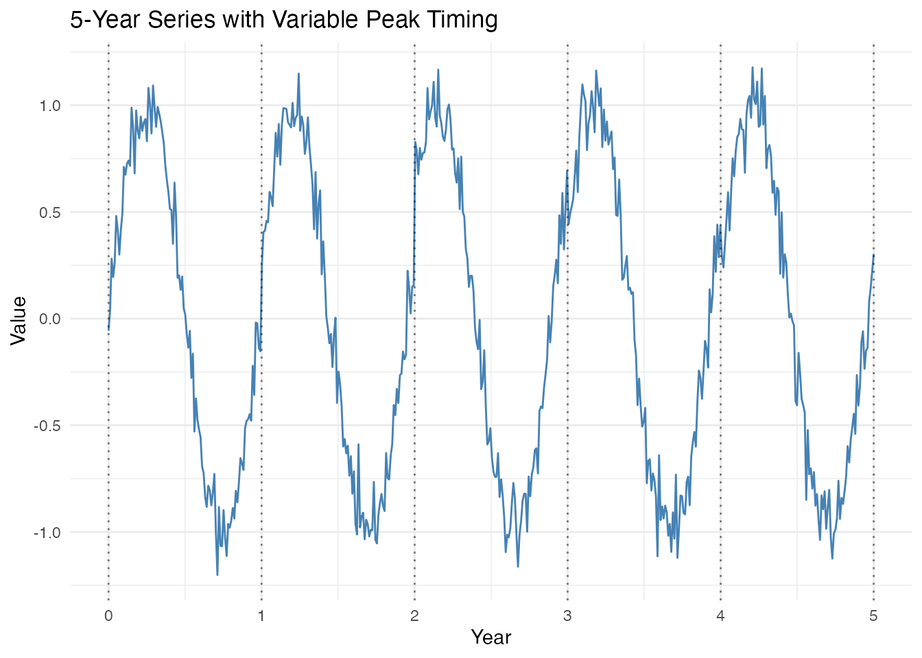

# Analyze peak timing
timing <- analyze.peak.timing(fd_short, period = period_short)
print(timing)
#> Peak Timing Variability Analysis
#> ---------------------------------
#> Number of peaks: 5
#> Mean timing:     0.1924
#> Std timing:      0.0364
#> Range timing:    0.1062
#> Variability:     0.3640 (moderate)
#> Timing trend:    -0.0110

Visualizing Peak Timing

# Get detected peaks with Fourier smoothing
peaks_short <- detect.peaks(fd_short, min_distance = 0.7,
                            smooth_first = TRUE, smooth_nbasis = NULL)
peak_df <- peaks_short$peaks[[1]]

# Plot with peaks marked
ggplot(df_short, aes(x = t, y = y)) +
  geom_line(color = "steelblue") +
  geom_point(data = peak_df, aes(x = time, y = value),
             color = "red", size = 3) +
  geom_vline(xintercept = 0:5, linetype = "dotted", alpha = 0.5) +
  labs(title = "5-Year Series with Detected Peaks",
       x = "Year", y = "Value")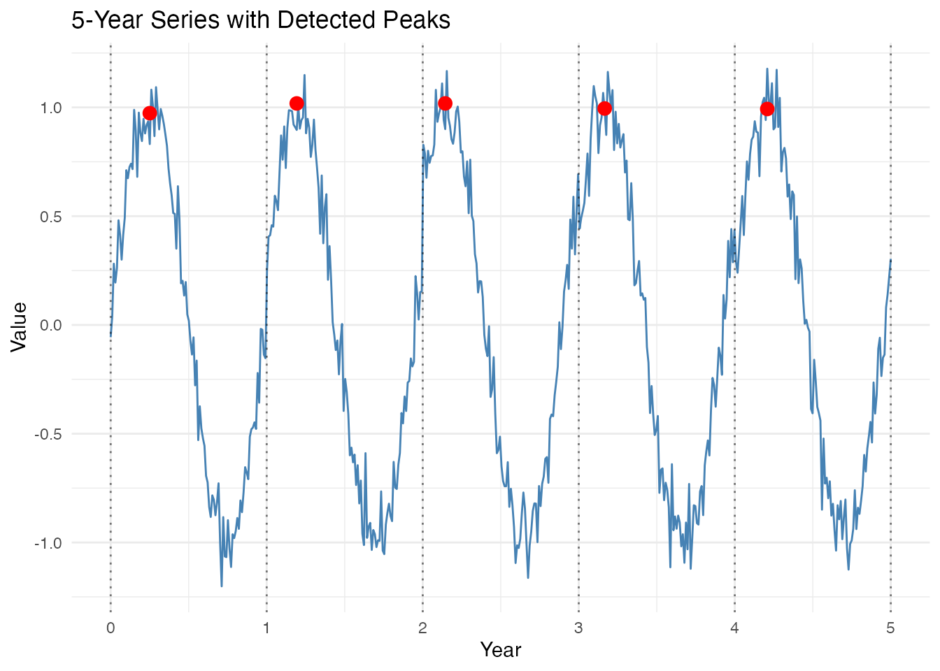

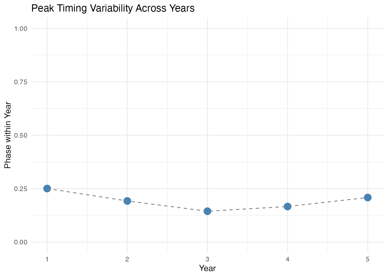
# Plot peak timing within each year
if (nrow(peak_df) >= 3) {
  peak_years <- floor(peak_df$time)
  peak_phase <- peak_df$time - peak_years

  df_timing <- data.frame(
    year = peak_years + 1,
    phase = peak_phase
  )

  ggplot(df_timing, aes(x = year, y = phase)) +
    geom_point(size = 4, color = "steelblue") +
    geom_line(linetype = "dashed", color = "gray50") +
    labs(title = "Peak Timing Variability Across Years",
         x = "Year", y = "Phase within Year") +
    ylim(0, 1)
}

Seasonality Classification

Automatically classify the type of seasonality pattern.

class_result <- classify.seasonality(fd_short, period = period_short)
print(class_result)
#> Seasonality Classification
#> --------------------------
#> Classification:   StableSeasonal
#> Is seasonal:      TRUE
#> Stable timing:    TRUE
#> Timing variability: 0.3640
#> Seasonal strength:  0.9351

# Visualize classification metrics
# Normalize timing variability to 0-1 scale (lower is better/more stable)
stability_score <- 1 - min(1, class_result$timing_variability / 0.2)

class_df <- data.frame(
  Metric = c("Seasonal Strength", "Timing Stability"),
  Value = c(class_result$seasonal_strength, stability_score)
)

ggplot(class_df, aes(x = Metric, y = Value, fill = Metric)) +
  geom_col() +
  ylim(0, 1) +
  labs(title = paste("Classification:", class_result$classification),
       x = "", y = "Score") +
  scale_fill_brewer(palette = "Set2") +
  theme(legend.position = "none")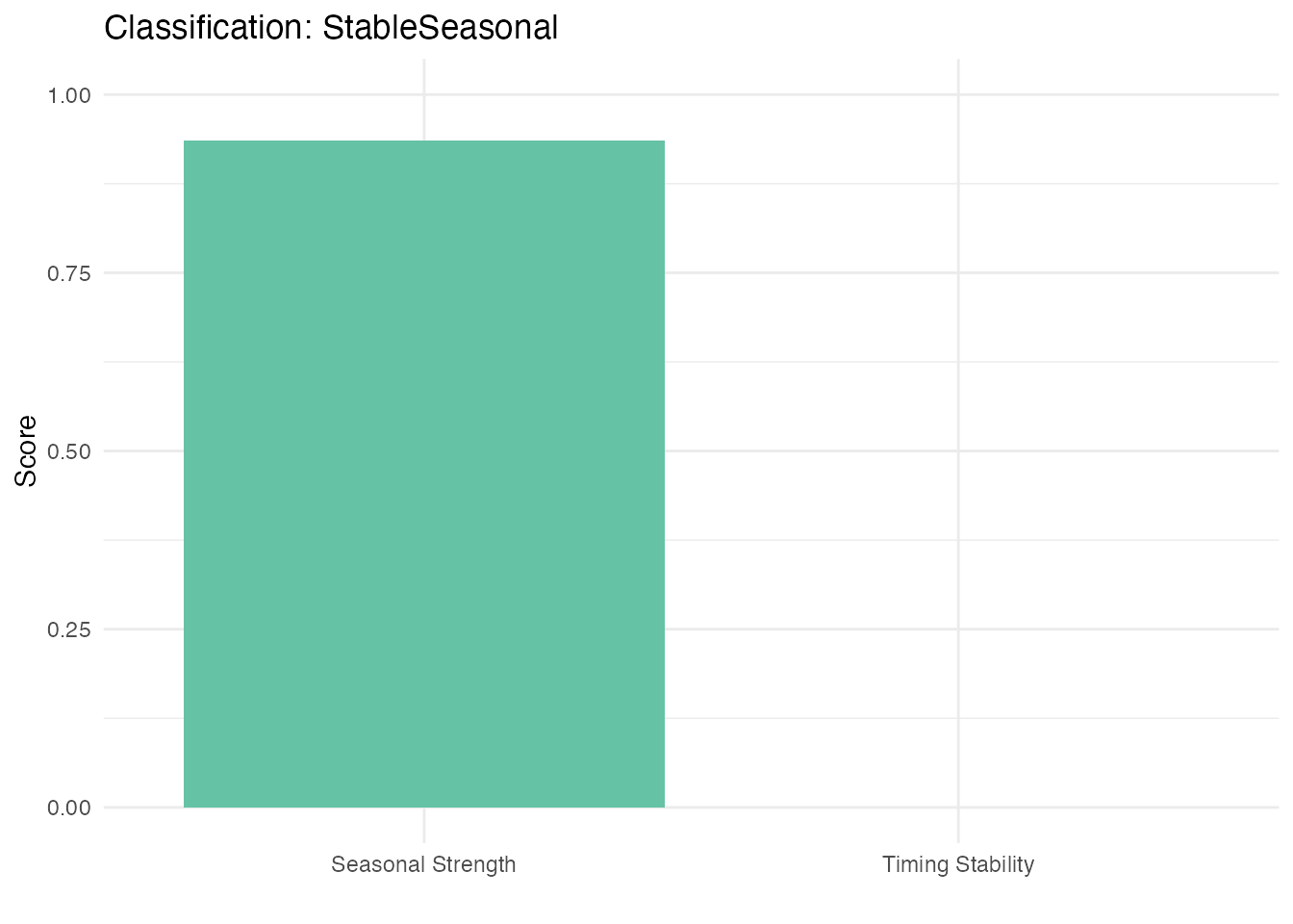

Classification Types

The classify.seasonality() function returns one of four classifications based on seasonal strength and timing variability:

Classification	Seasonal Strength	Timing Variability	Interpretation
stable	> 0.7	< 0.05	Consistent pattern across cycles
variable	0.4 - 0.7	0.05 - 0.15	Clear seasonality but parameters change
intermittent	< 0.4	any	Seasonality appears and disappears
none	< 0.2	any	No clear seasonal pattern

# Example: Stable seasonality - clean signal with consistent timing
X_stable <- sin(2 * pi * t_short / period_short) + rnorm(length(t_short), sd = 0.05)
fd_stable <- fdata(matrix(X_stable, nrow = 1), argvals = t_short)
class_stable <- classify.seasonality(fd_stable, period = period_short)

# Example: Variable seasonality - amplitude and timing drift
phase_var <- seq(0, 0.2, length.out = length(t_short))
amp_var <- 1 + 0.3 * sin(2 * pi * t_short / 3)
X_variable <- amp_var * sin(2 * pi * (t_short + phase_var) / period_short) +
              rnorm(length(t_short), sd = 0.2)
fd_variable <- fdata(matrix(X_variable, nrow = 1), argvals = t_short)
class_variable <- classify.seasonality(fd_variable, period = period_short)

# Example: Intermittent seasonality - pattern appears and disappears
X_intermittent <- ifelse(t_short < 2 | t_short > 4,
                         sin(2 * pi * t_short / period_short),
                         rnorm(sum(t_short >= 2 & t_short <= 4), sd = 0.5))
X_intermittent <- X_intermittent + rnorm(length(t_short), sd = 0.15)
fd_intermittent <- fdata(matrix(X_intermittent, nrow = 1), argvals = t_short)
class_intermittent <- classify.seasonality(fd_intermittent, period = period_short)

# Example: No seasonality - pure noise
X_none <- rnorm(length(t_short), sd = 1)
fd_none <- fdata(matrix(X_none, nrow = 1), argvals = t_short)
class_none <- classify.seasonality(fd_none, period = period_short)

# Summary
cat("Classification results:\n")
#> Classification results:
cat("  Stable signal:      ", class_stable$classification,
    "(strength:", round(class_stable$seasonal_strength, 2), ")\n")
#>   Stable signal:       StableSeasonal (strength: 0.99 )
cat("  Variable signal:    ", class_variable$classification,
    "(strength:", round(class_variable$seasonal_strength, 2), ")\n")
#>   Variable signal:     VariableTiming (strength: 0.78 )
cat("  Intermittent signal:", class_intermittent$classification,
    "(strength:", round(class_intermittent$seasonal_strength, 2), ")\n")
#>   Intermittent signal: IntermittentSeasonal (strength: 0.49 )
cat("  No seasonality:     ", class_none$classification,
    "(strength:", round(class_none$seasonal_strength, 2), ")\n")
#>   No seasonality:      NonSeasonal (strength: 0.01 )

# Visualize all four classification types
df_examples <- data.frame(
  t = rep(t_short, 4),
  y = c(X_stable, X_variable, X_intermittent, X_none),
  Type = factor(rep(c("Stable", "Variable", "Intermittent", "None"),
                    each = length(t_short)),
                levels = c("Stable", "Variable", "Intermittent", "None"))
)

ggplot(df_examples, aes(x = t, y = y)) +
  geom_line(color = "steelblue") +
  facet_wrap(~Type, ncol = 1, scales = "free_y") +
  labs(title = "Seasonality Classification Examples",
       x = "Time", y = "Value")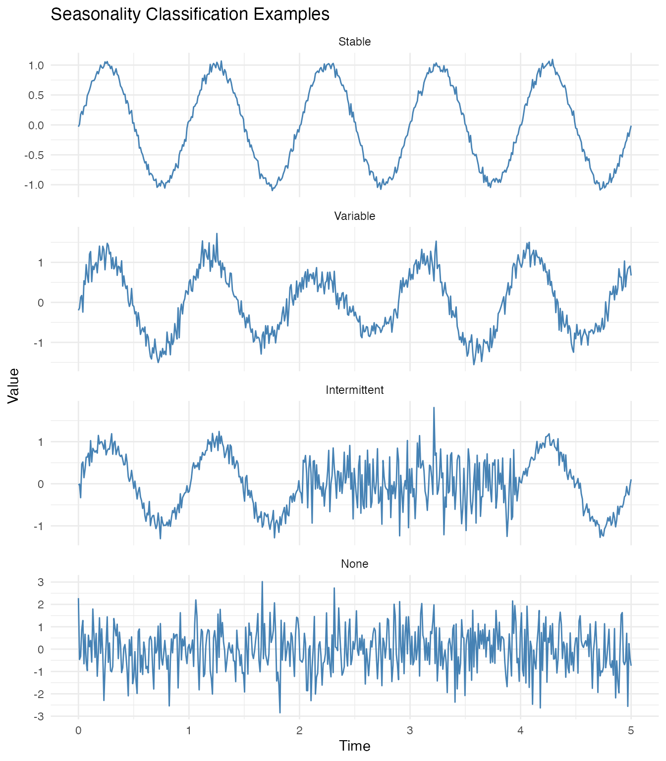

Automatic Fourier Smoothing for Short Series

Peak detection with automatic smoothing is especially important for noisy short series.

# More noisy short series
X_noisy_short <- sin(2 * pi * t_short / period_short) + rnorm(length(t_short), sd = 0.5)
fd_noisy_short <- fdata(matrix(X_noisy_short, nrow = 1), argvals = t_short)

# Auto-select smoothing via Fourier basis CV
cv_short <- fdata2basis_cv(fd_noisy_short, nbasis.range = 3:15, type = "fourier")
peaks_auto <- detect.peaks(cv_short$fitted, min_distance = 0.7)
cat("Peaks found with Fourier CV smoothing:", nrow(peaks_auto$peaks[[1]]), "\n")
#> Peaks found with Fourier CV smoothing: 5
cat("Expected peaks:", 5, "\n")
#> Expected peaks: 5
cat("Estimated period:", round(peaks_auto$mean_period, 3), "\n")
#> Estimated period: 0.997

Multiple Curves

All functions work with multiple curves simultaneously.

n_curves <- 5
t <- seq(0, 10, length.out = 200)
periods <- seq(1.8, 2.2, length.out = n_curves)  # Slightly varying periods

X <- matrix(0, n_curves, length(t))
for (i in 1:n_curves) {
  X[i, ] <- sin(2 * pi * t / periods[i]) + rnorm(length(t), sd = 0.2)
}

fd_curves <- fdata(X, argvals = t)

# Plot all curves
plot(fd_curves) +
  labs(title = "Multiple Seasonal Curves",
       x = "Time", y = "Value")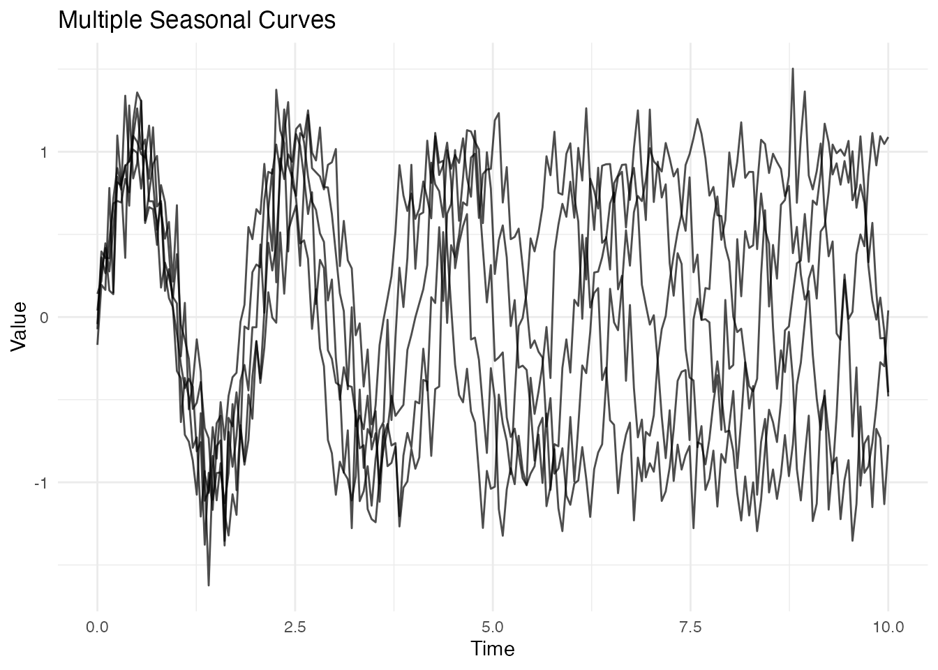

# Period estimation uses the mean curve
est_mean <- estimate.period(fd_curves, method = "fft")
cat("Estimated period (from mean):", est_mean$period, "\n")
#> Estimated period (from mean): 2.01005
cat("True mean period:", mean(periods), "\n")
#> True mean period: 2

# Peak detection for each curve
peaks_curves <- detect.peaks(fd_curves, min_distance = 1.5)
cat("\nMean period from peaks:", peaks_curves$mean_period, "\n")
#> 
#> Mean period from peaks: 1.730653

# Seasonal strength (aggregated)
ss_curves <- seasonal.strength(fd_curves, period = 2)
cat("Seasonal strength:", round(ss_curves, 3), "\n")
#> Seasonal strength: 0.557

Summary

Function Reference

Function	Purpose
estimate.period()	Estimate seasonal period (FFT or ACF method)
detect.periods()	Detect multiple concurrent periodicities
detect.peaks()	Find and characterize peaks (with auto GCV smoothing)
seasonal.strength()	Measure overall seasonality strength
seasonal.strength.curve()	Time-varying seasonality strength
detect.seasonality.changes()	Find onset/cessation of seasonality
detect.seasonality.changes.auto()	Auto threshold using Otsu’s method
instantaneous.period()	Period estimation for smoothly drifting signals
analyze.peak.timing()	Analyze peak timing variability across cycles
classify.seasonality()	Classify seasonality type (stable/variable/intermittent)
detrend()	Remove trends (linear, polynomial, LOESS, differencing)
decompose()	Seasonal-trend decomposition (additive or multiplicative)

Decision Guide

Non-stationary data (trends present):

• Linear trend: detrend(method = "linear") or use detrend_method = "linear" parameter
• Complex/curved trend: detrend(method = "loess") or method = "auto"
• Growing seasonal amplitude: decompose(method = "multiplicative")
• Full decomposition needed: decompose() returns trend + seasonal + remainder

Period estimation:

• Period unknown, signal stable: estimate.period(method = "fft")
• Period unknown, data has trend: estimate.period(detrend_method = "linear")
• Period unknown, multiple independent periods: detect.periods()
• Period varies smoothly over time: instantaneous.period()

Peak detection:

• Clean data: detect.peaks() with default parameters
• Noisy data: Add smooth_first = TRUE (Fourier smoothing with GCV-selected nbasis)
• Data with trend: Add detrend_method = "linear"
• Still too many peaks: Increase min_prominence

Seasonal strength:

• Single measurement: seasonal.strength()
• Data with trend: seasonal.strength(detrend_method = "linear")
• Track changes over time: seasonal.strength.curve()
• Detect when seasonality stops: detect.seasonality.changes.auto()

Short series (3-5 cycles):

• Characterize timing shifts: analyze.peak.timing()
• Classify pattern type: classify.seasonality()

Processing Large Numbers of Series

When analyzing many series (e.g., 500k time series), use a tiered approach to balance speed and depth of analysis:

Tier 1 - Fast screening (all series):

# Quick FFT period estimation - very fast
est <- estimate.period(fd, method = "fft")
if (est$confidence < 0.3) return("no_seasonality")

This filters out ~80% of series with no clear seasonality in typical mixed datasets.

Tier 2 - Validation (remaining ~20%):

# Add seasonal strength check
ss <- seasonal.strength(fd, period = est$period)
if (ss < 0.2) return("weak_seasonality")

Tier 3 - Full analysis (top candidates only):

# Expensive operations - classification, multiple periods
class <- classify.seasonality(fd, period = est$period)
periods <- detect.periods(fd)  # if multiple periods suspected

Parallelization:

All fdars Rust functions are thread-safe. Use parallel::mclapply() or future.apply::future_lapply() for parallel processing:

# Example batch processing workflow
library(parallel)
results <- mclapply(series_list, function(fd) {
  est <- estimate.period(fd, method = "fft")
  if (est$confidence < 0.3) return(list(classification = "none"))
  ss <- seasonal.strength(fd, period = est$period)
  list(period = est$period, confidence = est$confidence, strength = ss)
}, mc.cores = detectCores() - 1)

Memory management:

• Process in batches of 1000-5000 series
• Store only summary results (period, confidence, classification)
• Stream data from disk rather than loading all at once