Covariance Functions and Gaussian Process Generation • fdars

Introduction

Covariance functions (also called kernels) are fundamental building blocks for Gaussian processes. They define the correlation structure between function values at different points, controlling properties like smoothness and periodicity.

fdars provides a comprehensive set of covariance functions for generating synthetic functional data from Gaussian processes.

library(fdars)
#> 
#> Attaching package: 'fdars'
#> The following objects are masked from 'package:stats':
#> 
#>     cov, decompose, deriv, median, sd, var
#> The following object is masked from 'package:base':
#> 
#>     norm
library(ggplot2)
theme_set(theme_minimal())

Available Covariance Functions

Gaussian (Squared Exponential)

The most common choice, producing infinitely differentiable (very smooth) sample paths: $k(s, t) = \sigma^2 \exp\left(-\frac{(s-t)^2}{2\ell^2}\right)$

t <- seq(0, 1, length.out = 100)

# Create Gaussian covariance function
cov_gauss <- kernel.gaussian(variance = 1, length_scale = 0.2)
print(cov_gauss)
#> Covariance Kernel: gaussian 
#> Parameters:
#>    variance = 1 
#>    length_scale = 0.2

# Generate smooth GP samples
fd_gauss <- make.gaussian.process(n = 10, t = t, cov = cov_gauss, seed = 42)
plot(fd_gauss, main = "Gaussian Covariance (smooth)")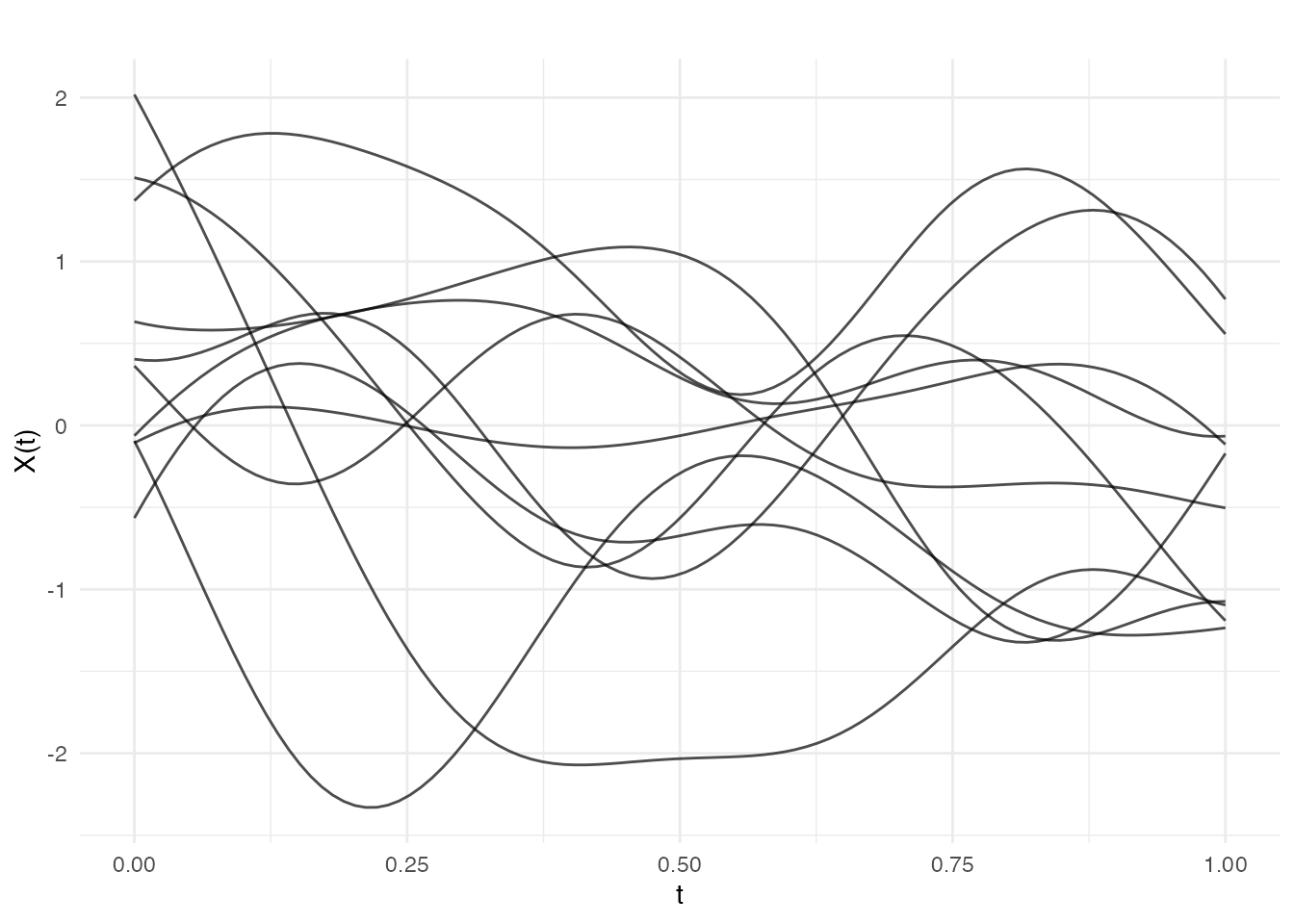

The length_scale parameter controls the correlation distance - smaller values produce more rapidly varying functions:

# Generate data for different length scales
ls_values <- c(0.05, 0.2, 0.5)
df_ls <- do.call(rbind, lapply(ls_values, function(ls) {
  fd <- make.gaussian.process(n = 5, t = t,
                              cov = kernel.gaussian(length_scale = ls),
                              seed = 42)
  data.frame(
    t = rep(t, 5),
    value = as.vector(t(fd$data)),
    curve = rep(1:5, each = length(t)),
    length_scale = paste("length_scale =", ls)
  )
}))
df_ls$length_scale <- factor(df_ls$length_scale,
                              levels = paste("length_scale =", ls_values))

ggplot(df_ls, aes(x = t, y = value, group = curve, color = factor(curve))) +
  geom_line(alpha = 0.8) +
  facet_wrap(~ length_scale) +
  labs(x = "t", y = "X(t)", title = "Effect of Length Scale") +
  theme_minimal() +
  theme(legend.position = "none")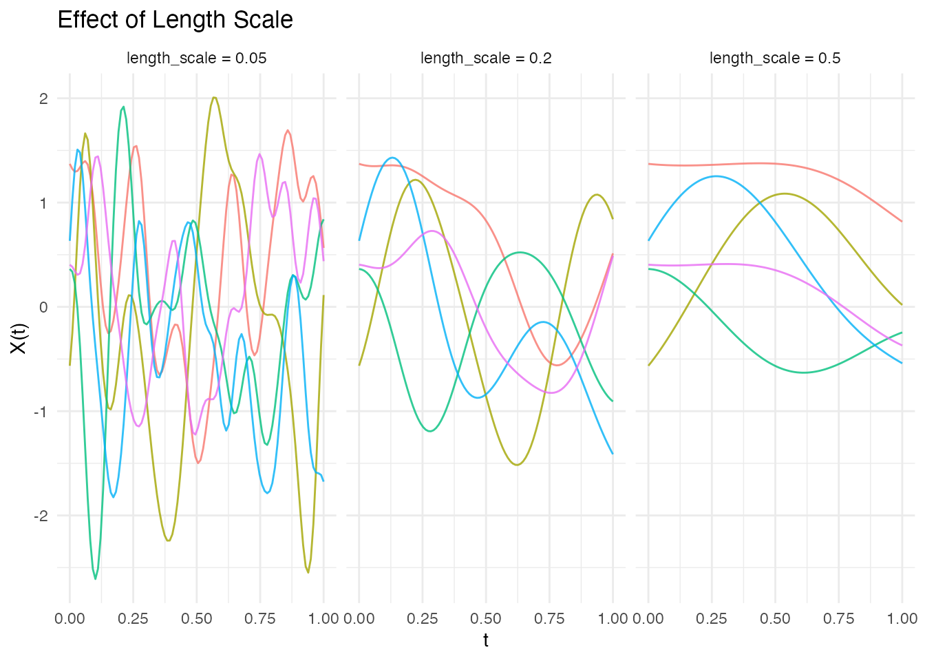

Exponential

Produces rougher paths than Gaussian (continuous but not differentiable): $k(s, t) = \sigma^2 \exp\left(-\frac{|s-t|}{\ell}\right)$

cov_exp <- kernel.exponential(variance = 1, length_scale = 0.2)
fd_exp <- make.gaussian.process(n = 10, t = t, cov = cov_exp, seed = 42)
plot(fd_exp, main = "Exponential Covariance (rough)")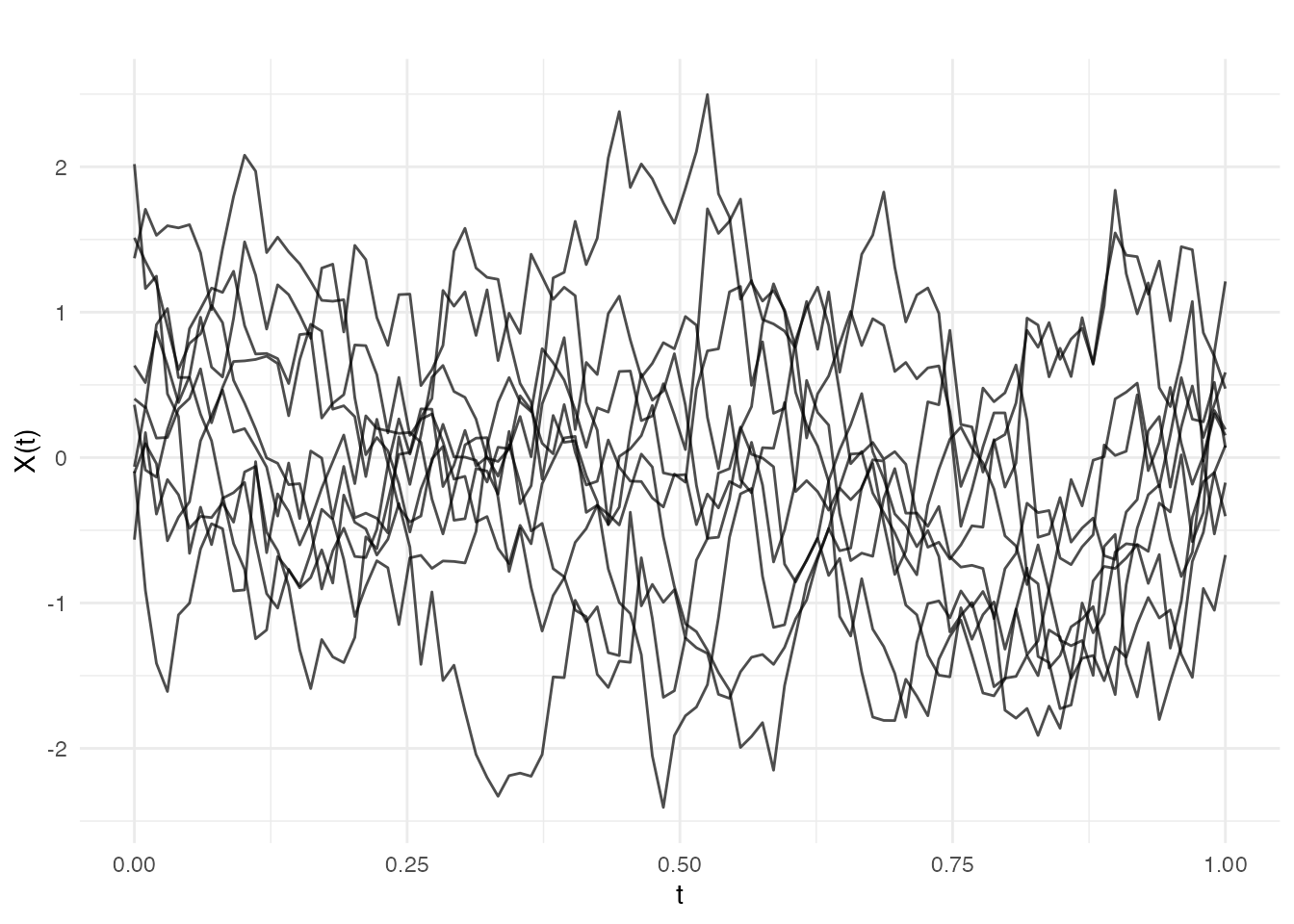

Matern Family

The Matern covariance is parameterized by smoothness parameter $\nu$ . It interpolates between Exponential ( $\nu = 0.5$ ) and Gaussian ( $\nu \to \infty$ ):

# Generate data for different nu values
nu_values <- c(0.5, 1.5, 2.5, Inf)
nu_labels <- c("0.5", "1.5", "2.5", "Inf")
df_matern <- do.call(rbind, lapply(seq_along(nu_values), function(i) {
  fd <- make.gaussian.process(n = 5, t = t,
                              cov = kernel.matern(length_scale = 0.2, nu = nu_values[i]),
                              seed = 42)
  data.frame(
    t = rep(t, 5),
    value = as.vector(t(fd$data)),
    curve = rep(1:5, each = length(t)),
    nu = paste("Matern nu =", nu_labels[i])
  )
}))
df_matern$nu <- factor(df_matern$nu,
                        levels = paste("Matern nu =", nu_labels))

ggplot(df_matern, aes(x = t, y = value, group = curve, color = factor(curve))) +
  geom_line(alpha = 0.8) +
  facet_wrap(~ nu, ncol = 2) +
  labs(x = "t", y = "X(t)", title = "Matern Covariance with Different Smoothness") +
  theme_minimal() +
  theme(legend.position = "none")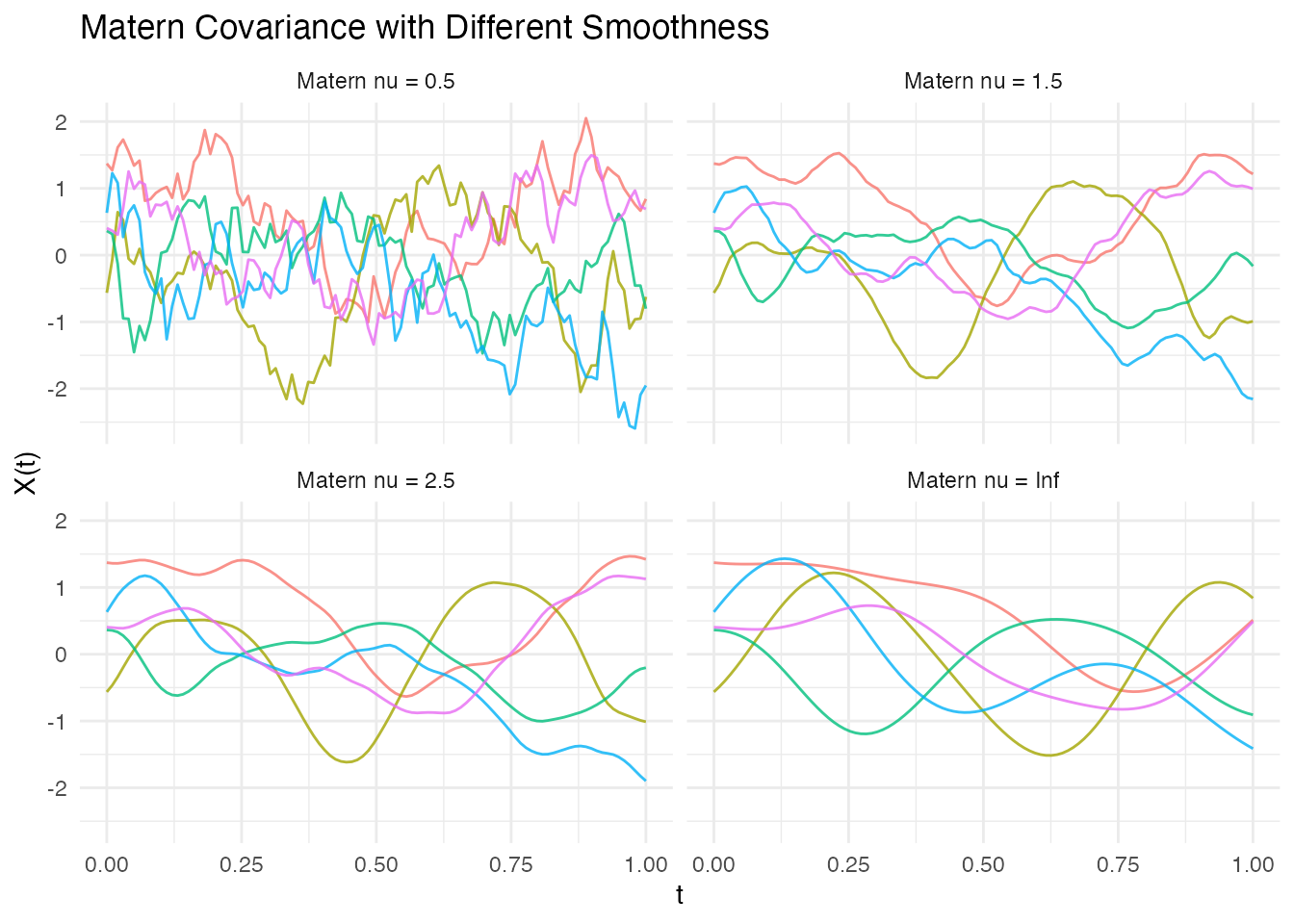

Common choices are: - $\nu = 0.5$ : Equivalent to Exponential (rough) - $\nu = 1.5$ : Once differentiable - $\nu = 2.5$ : Twice differentiable - $\nu = \infty$ : Equivalent to Gaussian (infinitely smooth)

Brownian Motion

Standard Brownian motion covariance: $k(s, t) = \sigma^2 \min(s, t)$

cov_brown <- kernel.brownian(variance = 1)
fd_brown <- make.gaussian.process(n = 10, t = t, cov = cov_brown, seed = 42)
plot(fd_brown, main = "Brownian Motion")

Note: Brownian covariance is only defined for 1D domains.

Periodic

For data with periodic structure: $k(s, t) = \sigma^2 \exp\left(-\frac{2\sin^2(\pi|s-t|/p)}{\ell^2}\right)$

t_long <- seq(0, 3, length.out = 200)
cov_per <- kernel.periodic(variance = 1, length_scale = 0.5, period = 1)
fd_per <- make.gaussian.process(n = 5, t = t_long, cov = cov_per, seed = 42)
plot(fd_per, main = "Periodic Covariance (period = 1)")

Linear

Linear covariance produces functions that are linear combinations of a constant and a linear function: $k(s, t) = \sigma^2 (s \cdot t + c)$

cov_lin <- kernel.linear(variance = 1, offset = 0)
fd_lin <- make.gaussian.process(n = 10, t = t, cov = cov_lin, seed = 42)
plot(fd_lin, main = "Linear Covariance")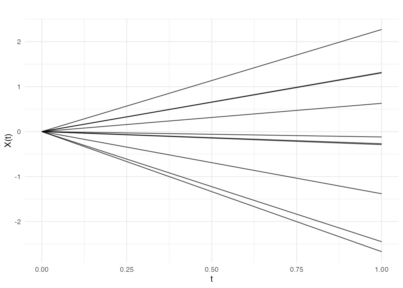

Polynomial

Generalization of linear to polynomial basis functions: $k(s, t) = \sigma^2 (s \cdot t + c)^d$

cov_poly <- kernel.polynomial(variance = 1, offset = 1, degree = 3)
fd_poly <- make.gaussian.process(n = 10, t = t, cov = cov_poly, seed = 42)
plot(fd_poly, main = "Polynomial Covariance (degree 3)")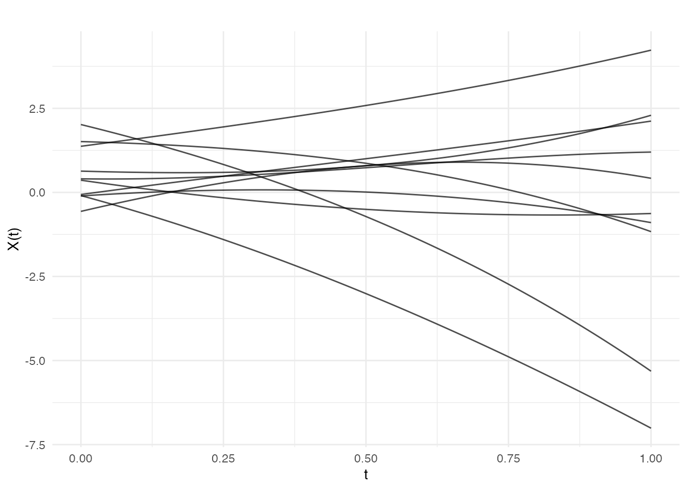

White Noise

Diagonal covariance representing independent noise: $k(s, t) = \sigma^2 \mathbf{1}_{s=t}$

cov_white <- kernel.whitenoise(variance = 0.5)
fd_white <- make.gaussian.process(n = 5, t = t, cov = cov_white, seed = 42)
plot(fd_white, main = "White Noise")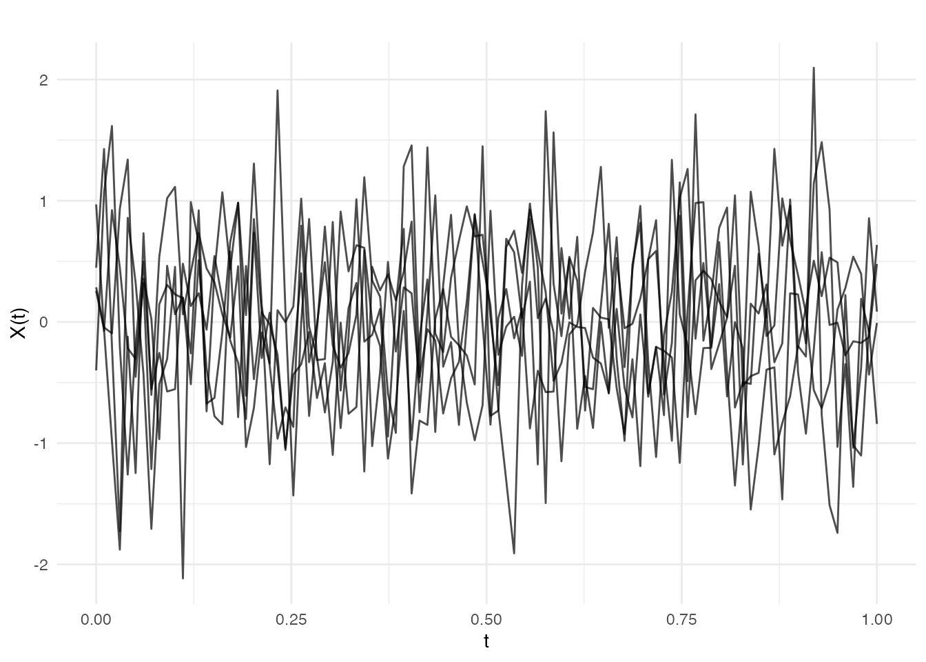

Combining Covariance Functions

Addition (kernel.add)

Sum of covariance functions models independent components:

# Signal + noise model
cov_signal <- kernel.gaussian(variance = 1, length_scale = 0.2)
cov_noise <- kernel.whitenoise(variance = 0.1)
cov_total <- kernel.add(cov_signal, cov_noise)

fd_noisy <- make.gaussian.process(n = 5, t = t, cov = cov_total, seed = 42)
plot(fd_noisy, main = "Smooth signal + noise")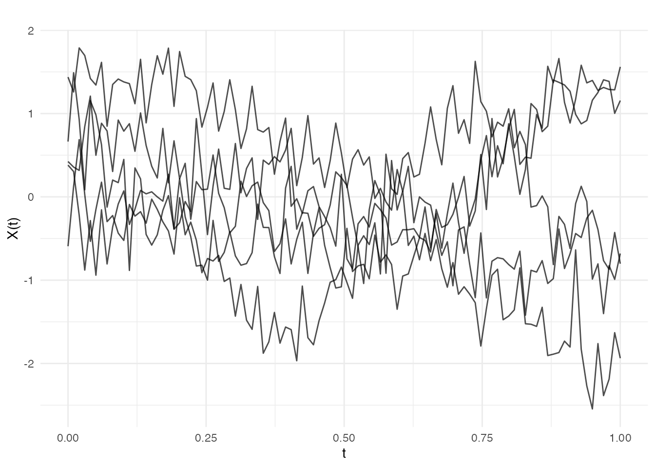

Multiplication (kernel.mult)

Product of covariance functions:

# Locally periodic: smooth envelope modulating periodic behavior
cov_envelope <- kernel.gaussian(variance = 1, length_scale = 0.5)
cov_periodic <- kernel.periodic(period = 0.2)
cov_local_per <- kernel.mult(cov_envelope, cov_periodic)

fd_local_per <- make.gaussian.process(n = 5, t = t, cov = cov_local_per, seed = 42)
plot(fd_local_per, main = "Locally periodic")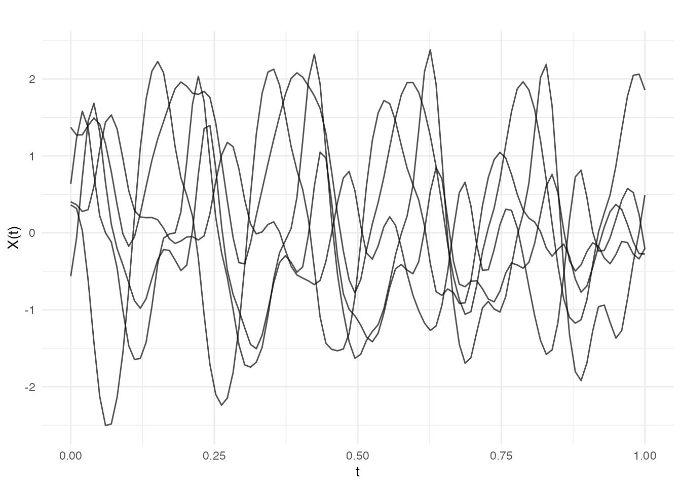

Mean Functions

Gaussian processes can have non-zero mean functions:

# Scalar mean
fd_mean5 <- make.gaussian.process(n = 10, t = t,
                                   cov = kernel.gaussian(variance = 0.1),
                                   mean = 5, seed = 42)
plot(fd_mean5, main = "Constant mean = 5")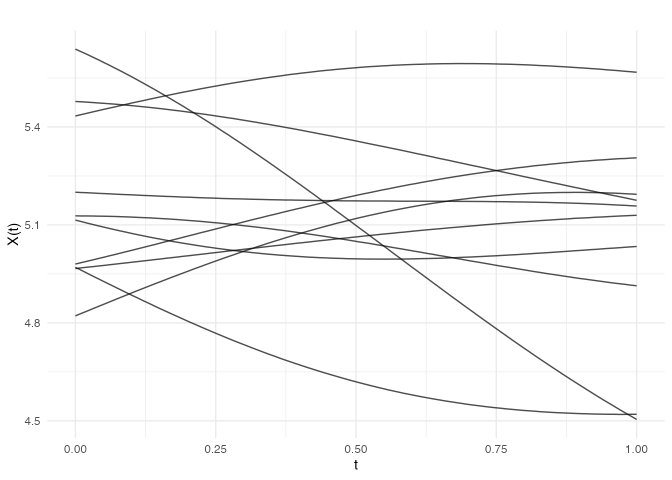


# Function mean
mean_func <- function(t) sin(2 * pi * t)
fd_sinmean <- make.gaussian.process(n = 10, t = t,
                                     cov = kernel.gaussian(variance = 0.1),
                                     mean = mean_func, seed = 42)
plot(fd_sinmean, main = "Sinusoidal mean function")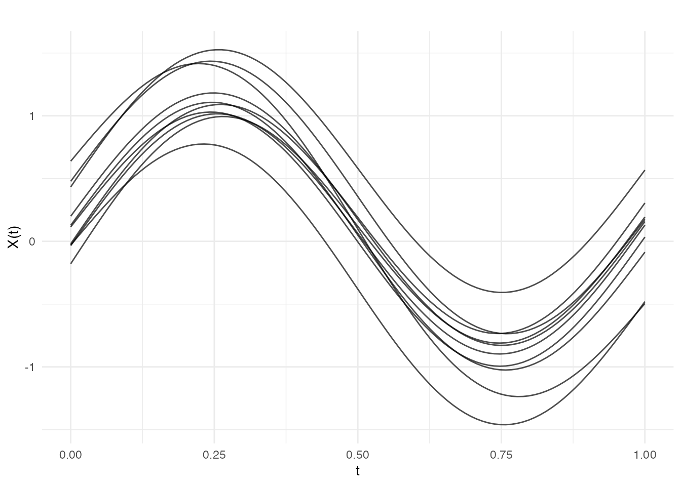

2D Functional Data (Surfaces)

Covariance functions can generate 2D functional data (surfaces):

s <- seq(0, 1, length.out = 30)
t2d <- seq(0, 1, length.out = 30)

# Generate 2D GP samples
fd2d <- make.gaussian.process(n = 4, t = list(s, t2d),
                               cov = kernel.gaussian(length_scale = 0.3),
                               seed = 42)
plot(fd2d)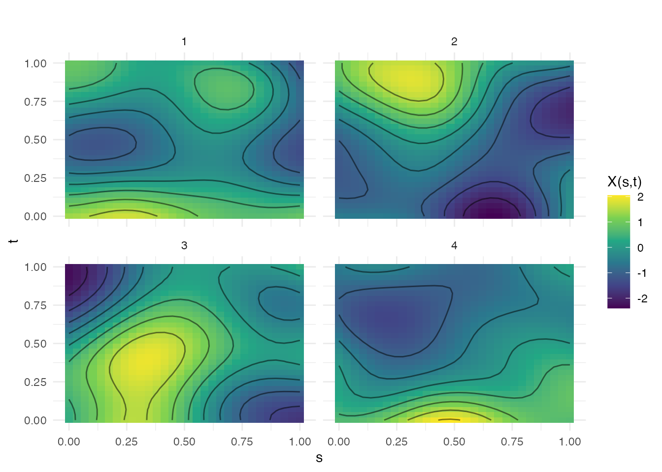

Note: kernel.brownian() and kernel.periodic() only support 1D domains.

Reproducibility

Use the seed parameter for reproducible samples:

fd1 <- make.gaussian.process(n = 3, t = t, cov = kernel.gaussian(), seed = 123)
fd2 <- make.gaussian.process(n = 3, t = t, cov = kernel.gaussian(), seed = 123)
all.equal(fd1$data, fd2$data)  # TRUE
#> [1] TRUE

Comparison of Smoothness

# Generate data for comparison
kernels <- list(
  list(name = "Gaussian (very smooth)", cov = kernel.gaussian()),
  list(name = "Matern 5/2", cov = kernel.matern(nu = 2.5)),
  list(name = "Matern 3/2", cov = kernel.matern(nu = 1.5)),
  list(name = "Exponential (rough)", cov = kernel.exponential())
)

df_smooth_comp <- do.call(rbind, lapply(kernels, function(k) {
  fd <- make.gaussian.process(n = 3, t = t, cov = k$cov, seed = 1)
  data.frame(
    t = rep(t, 3),
    value = as.vector(t(fd$data)),
    curve = rep(1:3, each = length(t)),
    kernel = k$name
  )
}))
df_smooth_comp$kernel <- factor(df_smooth_comp$kernel,
                                 levels = sapply(kernels, function(k) k$name))

ggplot(df_smooth_comp, aes(x = t, y = value, group = curve, color = factor(curve))) +
  geom_line(alpha = 0.8) +
  facet_wrap(~ kernel, ncol = 2) +
  labs(x = "t", y = "X(t)", title = "Comparison of Smoothness") +
  theme_minimal() +
  theme(legend.position = "none")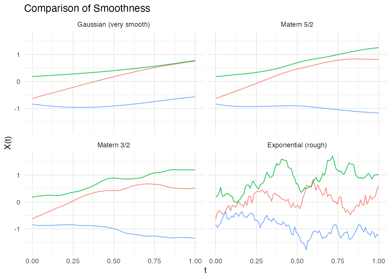

Summary Table

Covariance	Parameters	Smoothness	Notes
Gaussian	variance, length_scale	$C^\infty$	Most common, very smooth
Exponential	variance, length_scale	$C^0$	Rough, non-differentiable
Matern	variance, length_scale, nu	$C^{[\nu-1]}$	Flexible smoothness
Brownian	variance	$C^0$	1D only, non-stationary
Linear	variance, offset	-	Linear functions
Polynomial	variance, offset, degree	-	Polynomial functions
WhiteNoise	variance	-	Independent noise
Periodic	variance, length_scale, period	$C^\infty$	1D only, periodic

References

Rasmussen, C.E. and Williams, C.K.I. (2006). Gaussian Processes for Machine Learning. MIT Press.
Ramsay, J.O. and Silverman, B.W. (2005). Functional Data Analysis. Springer.