Functional Regression

Introduction

Functional regression extends classical regression to handle functional predictors or responses. The most common setting is scalar-on-function regression, where a scalar response $Y$ is predicted from a functional predictor $X(t)$.

The Functional Linear Model

The foundational model in functional regression is the functional linear model:

$$Y_i = \alpha + \int_{\mathcal{T}} \beta(t) X_i(t) \, dt + \epsilon_i$$

where:

• $Y_i$ is the scalar response for observation $i$
• $X_i(t)$ is the functional predictor observed over domain $\mathcal{T}$
• $\alpha$ is the intercept
• $\beta(t)$ is the coefficient function (unknown, to be estimated)
• $\epsilon_i \sim N(0, \sigma^2)$ are i.i.d. errors

The integral $\int \beta(t) X_i(t) \, dt$ can be interpreted as a weighted average of the functional predictor, where $\beta(t)$ determines the importance of each time point $t$ in predicting $Y$.

The Estimation Challenge

Unlike classical regression where we estimate a finite number of parameters, here we must estimate an entire function $\beta(t)$. This is an ill-posed inverse problem: infinitely many solutions may exist, and small changes in the data can lead to large changes in the estimate.

fdars provides three main approaches to regularize this problem:

1. Principal Component Regression (fregre.pc) — dimension reduction via FPCA
2. Basis Expansion Regression (fregre.basis) — represent $\beta(t)$ in a finite basis
3. Nonparametric Regression (fregre.np) — make no parametric assumptions

library(fdars)
#> 
#> Attaching package: 'fdars'
#> The following objects are masked from 'package:stats':
#> 
#>     cov, decompose, deriv, median, sd, var
#> The following object is masked from 'package:base':
#> 
#>     norm
library(ggplot2)
theme_set(theme_minimal())

# Generate example data
set.seed(42)
n <- 100
m <- 50
t_grid <- seq(0, 1, length.out = m)

# Functional predictors
X <- matrix(0, n, m)
for (i in 1:n) {
  X[i, ] <- sin(2 * pi * t_grid) * rnorm(1, 1, 0.3) +
            cos(4 * pi * t_grid) * rnorm(1, 0, 0.2) +
            rnorm(m, sd = 0.1)
}

fd <- fdata(X, argvals = t_grid)

# True coefficient function
beta_true <- sin(2 * pi * t_grid)

# Generate response: Y = integral(beta * X) + noise
y <- numeric(n)
for (i in 1:n) {
  y[i] <- sum(beta_true * X[i, ]) / m + rnorm(1, sd = 0.5)
}

plot(fd)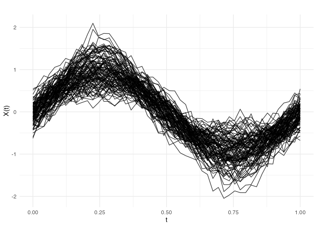

Principal Component Regression

Principal component regression (PCR) reduces the infinite-dimensional problem to a finite-dimensional one by projecting the functional data onto its principal components.

Mathematical Formulation

Using functional principal component analysis (FPCA), each curve can be represented as:

$$X_i(t) = \bar{X}(t) + \sum_{k=1}^{\infty} \xi_{ik} \phi_k(t)$$

where $\phi_k(t)$ are the eigenfunctions (principal components) and $\xi_{ik} = \int (X_i(t) - \bar{X}(t)) \phi_k(t) \, dt$ are the PC scores.

Truncating at $K$ components and substituting into the functional linear model gives:

$$Y_i = \alpha + \sum_{k=1}^{K} \gamma_k \xi_{ik} + \epsilon_i$$

where $\gamma_k = \int \beta(t) \phi_k(t) \, dt$. This is now a standard multiple linear regression with predictors $\xi_{i1}, \ldots, \xi_{iK}$.

The coefficient function is reconstructed as:

$$\hat{\beta}(t) = \sum_{k=1}^{K} \hat{\gamma}_k \phi_k(t)$$

Choosing the Number of Components

The key tuning parameter is $K$, the number of principal components:

• Too few: underfitting, missing important variation in $X(t)$
• Too many: overfitting, including noise components

Cross-validation or information criteria (AIC, BIC) can guide the choice.

Basic Usage

# Fit PC regression with 3 components
fit_pc <- fregre.pc(fd, y, ncomp = 3)
print(fit_pc)
#> Functional regression model
#>   Number of observations: 100 
#>   R-squared: 0.1682634

Examining the Fit

# Fitted values
fitted_pc <- fit_pc$fitted.values

# Residuals
residuals_pc <- y - fitted_pc

# R-squared
r2_pc <- 1 - sum(residuals_pc^2) / sum((y - mean(y))^2)
cat("R-squared:", round(r2_pc, 3), "\n")
#> R-squared: 0.168

Cross-Validation for Component Selection

# Find optimal number of components
cv_pc <- fregre.pc.cv(fd, y, kmax = 10)

cat("Optimal number of components:", cv_pc$ncomp.opt, "\n")
#> Optimal number of components:
cat("CV error by component:\n")
#> CV error by component:
print(round(cv_pc$cv.error, 4))
#>      1      2      3      4      5      6      7      8      9     10     11 
#> 0.2674 0.2700 0.2720 0.2735 0.2785 0.2735 0.2691 0.2718 0.2728 0.2744 0.2735 
#>     12     13     14     15 
#> 0.2746 0.2714 0.2703 0.2746

Prediction

# Split data
train_idx <- 1:80
test_idx <- 81:100

fd_train <- fd[train_idx, ]
fd_test <- fd[test_idx, ]
y_train <- y[train_idx]
y_test <- y[test_idx]

# Fit on training data
fit_train <- fregre.pc(fd_train, y_train, ncomp = 3)

# Predict on test data
y_pred <- predict(fit_train, fd_test)

# Evaluate
cat("Test RMSE:", round(pred.RMSE(y_test, y_pred), 3), "\n")
#> Test RMSE: 0.457
cat("Test R2:", round(pred.R2(y_test, y_pred), 3), "\n")
#> Test R2: 0.219

Basis Expansion Regression

Basis expansion regression represents both the functional predictor $X(t)$ and the coefficient function $\beta(t)$ using a finite set of basis functions, reducing the infinite-dimensional problem to a finite-dimensional one.

Mathematical Formulation

Let $\{B_j(t)\}_{j=1}^{J}$ be a set of basis functions (e.g., B-splines or Fourier). We expand:

$$X_i(t) = \sum_{j=1}^{J} c_{ij} B_j(t) \quad \text{and} \quad \beta(t) = \sum_{j=1}^{J} b_j B_j(t)$$

Substituting into the functional linear model:

$$Y_i = \alpha + \int \left(\sum_{j=1}^{J} b_j B_j(t)\right) \left(\sum_{k=1}^{J} c_{ik} B_k(t)\right) dt + \epsilon_i$$

This simplifies to:

$$Y_i = \alpha + \mathbf{c}_i^\top \mathbf{W} \mathbf{b} + \epsilon_i$$

where $\mathbf{c}_i = (c_{i1}, \ldots, c_{iJ})^\top$ are the basis coefficients of $X_i(t)$, $\mathbf{b} = (b_1, \ldots, b_J)^\top$ are the unknown coefficients of $\beta(t)$, and $\mathbf{W}$ is the inner product matrix with entries $W_{jk} = \int B_j(t) B_k(t) \, dt$.

Ridge Regularization

To prevent overfitting (especially with many basis functions), we add a roughness penalty. The penalized least squares objective is:

$$\min_{\alpha, \mathbf{b}} \sum_{i=1}^{n} \left(Y_i - \alpha - \mathbf{c}_i^\top \mathbf{W} \mathbf{b}\right)^2 + \lambda \int \left[\beta''(t)\right]^2 dt$$

The penalty $\int [\beta''(t)]^2 dt$ discourages rapid oscillations. In matrix form:

$$\min_{\alpha, \mathbf{b}} \|\mathbf{Y} - \alpha \mathbf{1} - \mathbf{C}\mathbf{W}\mathbf{b}\|^2 + \lambda \mathbf{b}^\top \mathbf{R} \mathbf{b}$$

where $\mathbf{R}$ is the roughness penalty matrix with $R_{jk} = \int B_j''(t) B_k''(t) \, dt$.

The solution is:

$$\hat{\mathbf{b}} = \left(\mathbf{W}^\top \mathbf{C}^\top \mathbf{C} \mathbf{W} + \lambda \mathbf{R}\right)^{-1} \mathbf{W}^\top \mathbf{C}^\top (\mathbf{Y} - \bar{Y})$$

Basis Choice

• B-splines: Flexible, local support, good for non-periodic data
• Fourier: Natural for periodic data, global support

Basic Usage

# Fit basis regression with 15 B-spline basis functions
fit_basis <- fregre.basis(fd, y, nbasis = 15, type = "bspline")
print(fit_basis)
#> Functional regression model
#>   Number of observations: 100 
#>   R-squared: 0.5805754

Regularization

The lambda parameter controls regularization:

# Higher lambda = more regularization
fit_basis_reg <- fregre.basis(fd, y, nbasis = 15, type = "bspline", lambda = 1)

Cross-Validation for Lambda

# Find optimal lambda
cv_basis <- fregre.basis.cv(fd, y, nbasis = 15, type = "bspline",
                            lambda = c(0, 0.001, 0.01, 0.1, 1, 10))

cat("Optimal lambda:", cv_basis$lambda.opt, "\n")
#> Optimal lambda:
cat("CV error by lambda:\n")
#> CV error by lambda:
print(round(cv_basis$cv.error, 4))
#>      0  0.001   0.01    0.1      1     10 
#> 0.5967 0.5926 0.5605 0.4299 0.3209 0.2977

Fourier Basis

For periodic data, use Fourier basis:

fit_fourier <- fregre.basis(fd, y, nbasis = 11, type = "fourier")

Nonparametric Regression

Nonparametric functional regression makes no parametric assumptions about the relationship between $X(t)$ and $Y$. Instead, it estimates $\mathbb{E}[Y | X = x]$ directly using local averaging techniques.

The General Framework

Given a new functional observation $X^*$, the predicted response is:

$$\hat{Y}^* = \hat{m}(X^*) = \sum_{i=1}^{n} w_i(X^*) Y_i$$

where $w_i(X^*)$ are weights that depend on the “distance” between $X^*$ and the training curves $X_i$. Different methods define these weights differently.

Functional Distance

A key component is the semimetric $d(X_i, X_j)$ measuring similarity between curves. Common choices:

• $L^2$ metric: $d(X_i, X_j) = \sqrt{\int [X_i(t) - X_j(t)]^2 \, dt}$
• $L^p$ metric: $d(X_i, X_j) = \left(\int |X_i(t) - X_j(t)|^p \, dt\right)^{1/p}$
• PCA-based semimetric: $d(X_i, X_j) = \sqrt{\sum_{k=1}^{K} (\xi_{ik} - \xi_{jk})^2}$ using PC scores

Nadaraya-Watson Estimator

The Nadaraya-Watson (kernel regression) estimator uses:

$$\hat{m}(X^*) = \frac{\sum_{i=1}^{n} K\left(\frac{d(X^*, X_i)}{h}\right) Y_i}{\sum_{i=1}^{n} K\left(\frac{d(X^*, X_i)}{h}\right)}$$

where $K(\cdot)$ is a kernel function and $h > 0$ is the bandwidth controlling the smoothness:

• Small $h$: weights concentrated on nearest neighbors (low bias, high variance)
• Large $h$: weights spread across many observations (high bias, low variance)

Common kernels include:

Kernel	Formula $K(u)$
Gaussian	$\frac{1}{\sqrt{2\pi}} e^{-u^2/2}$
Epanechnikov	$\frac{3}{4}(1-u^2) \mathbf{1}_{|u| \leq 1}$
Uniform	$\frac{1}{2} \mathbf{1}_{|u| \leq 1}$

k-Nearest Neighbors

The k-NN estimator averages the responses of the $k$ closest curves:

$$\hat{m}(X^*) = \frac{1}{k} \sum_{i \in \mathcal{N}_k(X^*)} Y_i$$

where $\mathcal{N}_k(X^*)$ is the set of indices of the $k$ nearest neighbors of $X^*$.

Two variants are available:

• Global k-NN (kNN.gCV): single $k$ selected by leave-one-out cross-validation
• Local k-NN (kNN.lCV): adaptive $k$ that may vary per prediction point

Nadaraya-Watson Example

# Fit nonparametric regression with Nadaraya-Watson
fit_np <- fregre.np(fd, y, type.S = "S.NW")
print(fit_np)
#> Nonparametric functional regression model
#>   Number of observations: 100 
#>   Smoother type: S.NW 
#>   Bandwidth: 0.3302789 
#>   R-squared: 0.0552

k-Nearest Neighbors

Two flavors of k-NN are available:

# Global k-NN (single k for all observations)
fit_knn_global <- fregre.np(fd, y, type.S = "kNN.gCV")

# Local k-NN (adaptive k per observation)
fit_knn_local <- fregre.np(fd, y, type.S = "kNN.lCV")

cat("Global k-NN optimal k:", fit_knn_global$knn, "\n")
#> Global k-NN optimal k: 20

Bandwidth Selection

# Cross-validation for bandwidth
cv_np <- fregre.np.cv(fd, y, h.seq = seq(0.1, 1, by = 0.1))

cat("Optimal bandwidth:", cv_np$h.opt, "\n")
#> Optimal bandwidth:

Different Kernels

# Epanechnikov kernel
fit_epa <- fregre.np(fd, y, Ker = "epa")

# Available kernels: "norm", "epa", "tri", "quar", "cos", "unif"

Different Metrics

# Use L1 metric instead of default L2
fit_np_l1 <- fregre.np(fd, y, metric = metric.lp, p = 1)

# Use semimetric based on PCA
fit_np_pca <- fregre.np(fd, y, metric = semimetric.pca, ncomp = 5)

Comparing Methods

# Fit all methods on training data
fit1 <- fregre.pc(fd_train, y_train, ncomp = 3)
fit2 <- fregre.basis(fd_train, y_train, nbasis = 15)
fit3 <- fregre.np(fd_train, y_train, type.S = "kNN.gCV")

# Predict on test data
pred1 <- predict(fit1, fd_test)
pred2 <- predict(fit2, fd_test)
pred3 <- predict(fit3, fd_test)

# Compare performance
results <- data.frame(
  Method = c("PC Regression", "Basis Regression", "k-NN"),
  RMSE = c(pred.RMSE(y_test, pred1),
           pred.RMSE(y_test, pred2),
           pred.RMSE(y_test, pred3)),
  R2 = c(pred.R2(y_test, pred1),
         pred.R2(y_test, pred2),
         pred.R2(y_test, pred3))
)
print(results)
#>             Method      RMSE          R2
#> 1    PC Regression 0.4570245  0.21884391
#> 2 Basis Regression 0.8989962 -2.02255778
#> 3             k-NN 0.4935318  0.08906132

Visualizing Predictions

# Create comparison data frame
df_pred <- data.frame(
  Observed = y_test,
  PC = pred1,
  Basis = pred2,
  kNN = pred3
)

# Observed vs predicted
ggplot(df_pred, aes(x = Observed, y = PC)) +
  geom_point() +
  geom_abline(intercept = 0, slope = 1, linetype = "dashed", color = "red") +
  labs(title = "PC Regression: Observed vs Predicted",
       x = "Observed", y = "Predicted") +
  theme_minimal()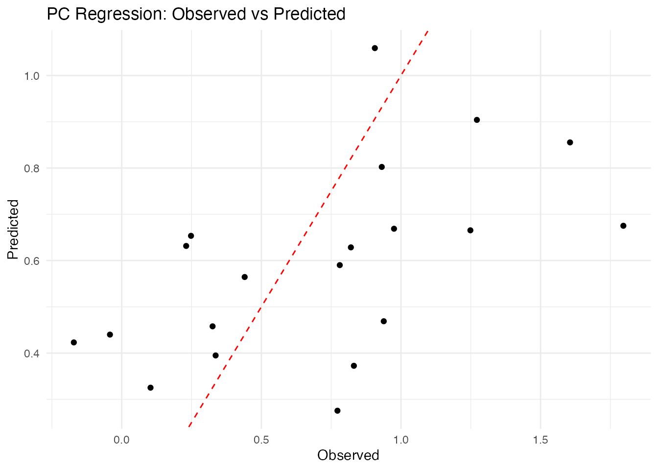

Method Selection Guide

When to Use Each Method

Principal Component Regression (fregre.pc):

• Best when the functional predictor has clear dominant modes of variation
• Computationally efficient for large datasets
• Interpretable: each PC represents a pattern in the data
• Use when $n$ is small relative to the complexity of $X(t)$

Basis Expansion Regression (fregre.basis):

• Best when you believe $\beta(t)$ is smooth
• Use B-splines for local features, Fourier for periodic patterns
• The penalty parameter $\lambda$ provides automatic regularization
• Good when you want to visualize and interpret $\hat{\beta}(t)$

Nonparametric Regression (fregre.np):

• Best when the relationship between $X$ and $Y$ may be nonlinear
• Makes minimal assumptions about the data-generating process
• Computationally more expensive (requires distance calculations)
• May require larger sample sizes for stable estimation

Comparison Table

Method	Model	Key Parameter	Computation	Interpretability
PC Regression	$Y = \alpha + \sum_k \gamma_k \xi_{ik}$	$K$ (# components)	Fast	High
Basis Regression	$Y = \alpha + \int \beta(t) X(t) dt$	$\lambda$ (penalty)	Fast	High
Nadaraya-Watson	$Y = m(X)$ (nonparametric)	$h$ (bandwidth)	Moderate	Low
k-NN	$Y = \frac{1}{k}\sum_{j \in \mathcal{N}_k} Y_j$	$k$ (neighbors)	Moderate	Low

Prediction Metrics

Model performance is evaluated using standard regression metrics. Given observed values $y_1, \ldots, y_n$ and predictions $\hat{y}_1, \ldots, \hat{y}_n$:

Metric	Formula	Interpretation
MAE	$\frac{1}{n}\sum_{i=1}^n |y_i - \hat{y}_i|$	Average absolute error
MSE	$\frac{1}{n}\sum_{i=1}^n (y_i - \hat{y}_i)^2$	Average squared error
RMSE	$\sqrt{\text{MSE}}$	Error in original units
$R^2$	$1 - \frac{\sum(y_i - \hat{y}_i)^2}{\sum(y_i - \bar{y})^2}$	Proportion of variance explained

# Available metrics for model evaluation
cat("MAE:", pred.MAE(y_test, pred1), "\n")
#> MAE: 0.3819577
cat("MSE:", pred.MSE(y_test, pred1), "\n")
#> MSE: 0.2088714
cat("RMSE:", pred.RMSE(y_test, pred1), "\n")
#> RMSE: 0.4570245
cat("R2:", pred.R2(y_test, pred1), "\n")
#> R2: 0.2188439

Cross-Validation

All methods support leave-one-out cross-validation (LOOCV) for parameter selection:

$$\text{CV} = \frac{1}{n} \sum_{i=1}^{n} (Y_i - \hat{Y}_{-i})^2$$

where $\hat{Y}_{-i}$ is the prediction for observation $i$ when it is left out of the training set. This is implemented efficiently using the “hat matrix trick” for linear methods.

References

Foundational texts:

• Ramsay, J.O. and Silverman, B.W. (2005). Functional Data Analysis, 2nd ed. Springer.
• Ferraty, F. and Vieu, P. (2006). Nonparametric Functional Data Analysis: Theory and Practice. Springer.
• Horváth, L. and Kokoszka, P. (2012). Inference for Functional Data with Applications. Springer.

Key methodological papers:

• Cardot, H., Ferraty, F., and Sarda, P. (1999). Functional Linear Model. Statistics & Probability Letters, 45(1), 11-22.
• Reiss, P.T. and Ogden, R.T. (2007). Functional Principal Component Regression and Functional Partial Least Squares. Journal of the American Statistical Association, 102(479), 984-996.
• Goldsmith, J., Bobb, J., Crainiceanu, C., Caffo, B., and Reich, D. (2011). Penalized Functional Regression. Journal of Computational and Graphical Statistics, 20(4), 830-851.

On nonparametric functional regression:

• Ferraty, F., Laksaci, A., and Vieu, P. (2006). Estimating Some Characteristics of the Conditional Distribution in Nonparametric Functional Models. Statistical Inference for Stochastic Processes, 9, 47-76.