Working with Irregular Functional Data • fdars

library(fdars)
#> 
#> Attaching package: 'fdars'
#> The following objects are masked from 'package:stats':
#> 
#>     cov, decompose, deriv, median, sd, var
#> The following object is masked from 'package:base':
#> 
#>     norm
library(ggplot2)
theme_set(theme_minimal())

Introduction

Many real-world functional data are irregularly sampled, meaning:

Different curves are observed at different time points
Observations may be sparse (few points per curve)
Sampling density may vary within or across curves

The fdars package provides the irregFdata class to handle such data naturally, avoiding the need for imputation or interpolation before analysis.

Common Applications

Longitudinal studies: Patients visited at different times
Sensor data: Measurements with gaps or varying frequency
Environmental monitoring: Non-uniform temporal sampling
Financial data: Trades occurring at irregular intervals

The irregFdata Class

Creating irregFdata Objects

An irregFdata object stores observation times and values as lists:

# Three curves with different observation points
argvals <- list(
  c(0.0, 0.3, 0.7, 1.0),       # 4 points
  c(0.0, 0.2, 0.4, 0.6, 0.8, 1.0),  # 6 points
  c(0.1, 0.5, 0.9)              # 3 points
)

X <- list(
  c(0.1, 0.5, 0.3, 0.2),
  c(0.0, 0.4, 0.8, 0.6, 0.4, 0.1),
  c(0.3, 0.7, 0.2)
)

ifd <- irregFdata(argvals, X)
print(ifd)
#> Irregular Functional Data Object
#> =================================
#>   Number of observations: 3 
#>   Points per curve:
#>     Min: 3 
#>     Median: 4 
#>     Max: 6 
#>     Total: 13 
#>   Domain: [ 0 , 1 ]

Structure

# Number of observations
ifd$n
#> [1] 3

# Observation counts per curve
sapply(ifd$X, length)
#> [1] 4 6 3

# Domain range
ifd$rangeval
#> [1] 0 1

Checking Data Type

# Regular fdata
fd_regular <- fdata(matrix(rnorm(100), 10, 10))
is.irregular(fd_regular)
#> [1] FALSE

# Irregular fdata
is.irregular(ifd)
#> [1] TRUE

Sparsifying Regular Data

Use sparsify() to convert regular fdata to irregFdata:

# Start with regular data
t <- seq(0, 1, length.out = 100)
fd <- simFunData(n = 10, argvals = t, M = 5, seed = 42)

# Create sparse version with 15-30 observations per curve
ifd <- sparsify(fd, minObs = 15, maxObs = 30, seed = 123)
print(ifd)
#> Irregular Functional Data Object
#> =================================
#>   Number of observations: 10 
#>   Points per curve:
#>     Min: 16 
#>     Median: 26.5 
#>     Max: 30 
#>     Total: 243 
#>   Domain: [ 0 , 1 ]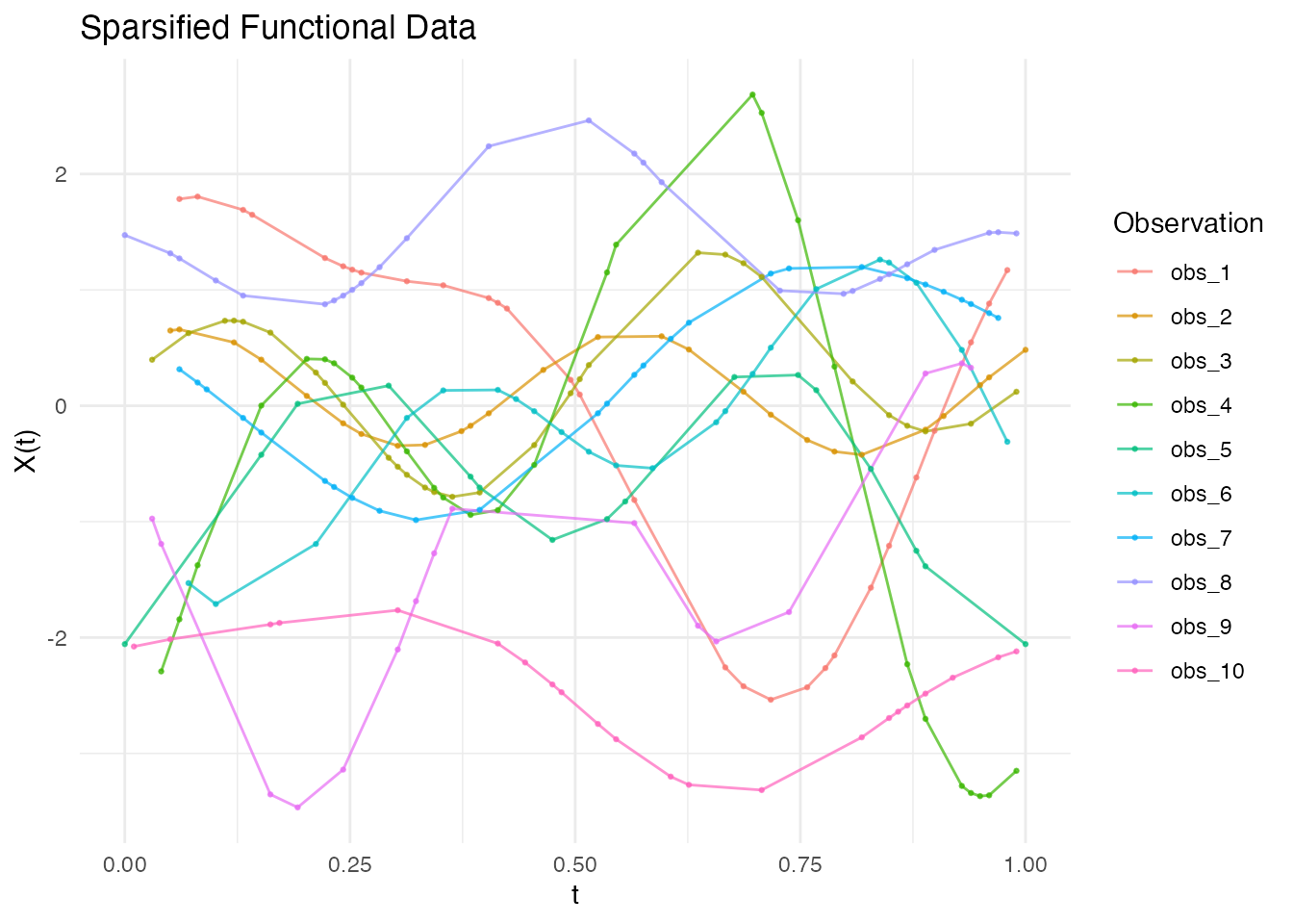

Visualizing Sparse Data

autoplot(ifd) +
  labs(title = "Sparsified Functional Data")

Non-Uniform Sparsification

Control sampling density with a probability function:

# More observations in the middle
prob_middle <- function(t) dnorm(t, mean = 0.5, sd = 0.2)

# More observations at the edges (U-shaped probability)
prob_edges <- function(t) 0.1 + 4 * (t - 0.5)^2

fd <- simFunData(n = 20, argvals = t, M = 5, seed = 42)

ifd_uniform <- sparsify(fd, minObs = 15, maxObs = 25, seed = 123)
ifd_middle <- sparsify(fd, minObs = 15, maxObs = 25, prob = prob_middle, seed = 123)
ifd_edges <- sparsify(fd, minObs = 15, maxObs = 25, prob = prob_edges, seed = 123)

p1 <- autoplot(ifd_uniform) + labs(title = "Uniform Sampling")
p2 <- autoplot(ifd_middle) + labs(title = "Dense in Middle")
p3 <- autoplot(ifd_edges) + labs(title = "Dense at Edges")
gridExtra::grid.arrange(p1, p2, p3, ncol = 1)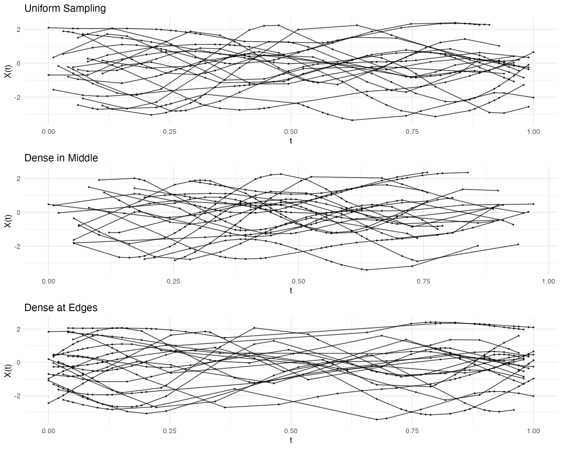

Converting to Regular Grid

Use as.fdata() to convert back to regular fdata:

Method: NA Fill

Only exact matches are filled; other points get NA:

ifd <- sparsify(fd[1:3], minObs = 10, maxObs = 20, seed = 123)

fd_na <- as.fdata(ifd, method = "na")

# Show some data with NAs
fd_na$data[1, 1:20]
#>  [1]         NA  1.7304109         NA  2.0573334         NA         NA
#>  [7]  1.2834072         NA         NA         NA         NA         NA
#> [13]         NA -1.1737028 -1.2287149 -1.2131357         NA -0.7393675
#> [19]         NA         NA

Method: Linear Interpolation

Interpolate between observed points:

# Specify target grid
target_grid <- seq(0, 1, length.out = 50)
fd_interp <- as.fdata(ifd, argvals = target_grid, method = "linear")

# No NAs within observed range
sum(is.na(fd_interp$data))
#> [1] 19

p1 <- autoplot(ifd[1]) + labs(title = "Original Sparse Data (1 curve)")
p2 <- autoplot(fd_interp[1]) + labs(title = "After Linear Interpolation")
gridExtra::grid.arrange(p1, p2, ncol = 2)
#> Warning: Removed 4 rows containing missing values or values outside the scale range
#> (`geom_line()`).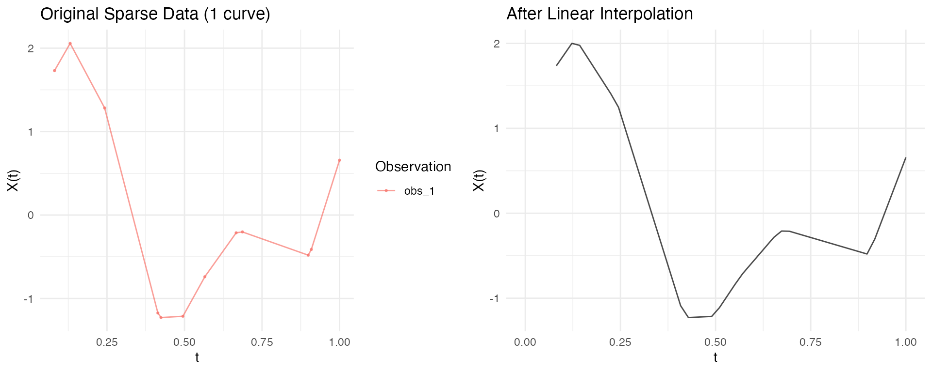

Basis Representation for Sparse Data

Basis representation is a powerful approach for handling irregular/sparse functional data:

Smooth noisy observations
Reduce dimensionality (from many observation points to few coefficients)
Regularize the curves for downstream analysis (FPCA, regression, clustering)
Convert irregular data to regular representation

For comprehensive coverage of basis functions, see vignette("basis-representation").

Direct Basis Fitting (Recommended)

The preferred approach for irregular data is to fit basis functions directly to each curve’s observation points using least squares. This avoids interpolation artifacts and handles varying observation densities naturally.

# Create sparse/irregular data
t <- seq(0, 1, length.out = 100)
fd_sim <- simFunData(n = 10, argvals = t, M = 5, seed = 42)
ifd <- sparsify(fd_sim, minObs = 15, maxObs = 30, seed = 123)

# Fit basis directly to irregular data (no interpolation needed!)
coefs <- fdata2basis(ifd, nbasis = 10, type = "bspline")

# Reconstruct on any target grid
fd_smooth <- basis2fdata(coefs, argvals = t, type = "bspline")

# Compare sparse observations vs smooth reconstruction
p1 <- autoplot(ifd[1:3], alpha = 0.8) +
  labs(title = "Sparse Observations (3 curves)")
p2 <- autoplot(fd_smooth[1:3], alpha = 0.8) +
  labs(title = "Basis Reconstruction")
gridExtra::grid.arrange(p1, p2, ncol = 2)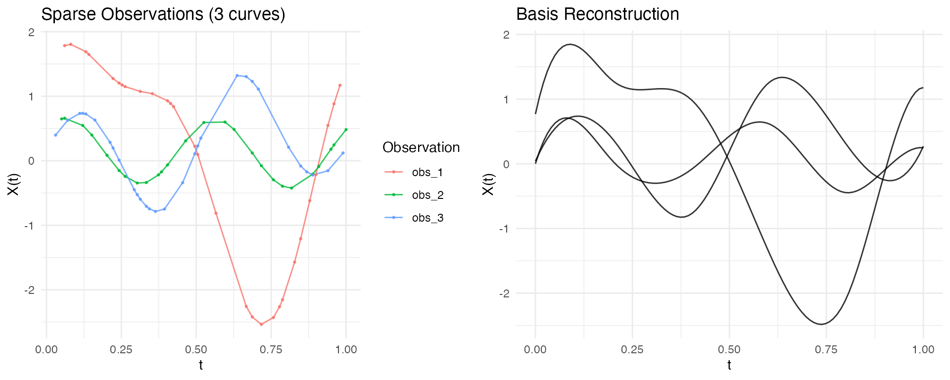

This approach works with both B-spline and Fourier bases:

# Fourier basis for periodic patterns
coefs_fourier <- fdata2basis(ifd, nbasis = 9, type = "fourier")
fd_fourier <- basis2fdata(coefs_fourier, argvals = t, type = "fourier")

autoplot(fd_fourier[1:5], alpha = 0.8) +
  labs(title = "Fourier Basis Reconstruction (9 basis)")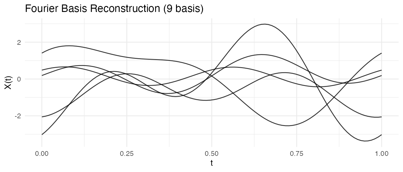

Comparing Approaches: Direct vs Interpolate-Then-Fit

Let’s compare the two approaches. The key advantage of direct fitting is that it works even when observations don’t cover the full domain:

# Create sparse data with known ground truth
t <- seq(0, 1, length.out = 100)
fd_true <- simFunData(n = 5, argvals = t, M = 5, seed = 42)
ifd <- sparsify(fd_true, minObs = 15, maxObs = 25, seed = 456)

# Show observation coverage
cat("Observation ranges per curve:\n")
#> Observation ranges per curve:
for (i in 1:5) {
  r <- range(ifd$argvals[[i]])
  cat(sprintf("  Curve %d: [%.2f, %.2f] (%d observations)\n",
              i, r[1], r[2], length(ifd$argvals[[i]])))
}
#>   Curve 1: [0.07, 0.90] (19 observations)
#>   Curve 2: [0.03, 1.00] (23 observations)
#>   Curve 3: [0.03, 0.99] (21 observations)
#>   Curve 4: [0.04, 0.90] (25 observations)
#>   Curve 5: [0.00, 1.00] (22 observations)

# APPROACH 1: Direct basis fitting - works on full domain
coefs_direct <- fdata2basis(ifd, nbasis = 12, type = "bspline")
fd_direct <- basis2fdata(coefs_direct, argvals = t, type = "bspline")

# APPROACH 2: Interpolate first - only works within observed range
fd_interp <- as.fdata(ifd, argvals = t, method = "linear")
cat("\nNAs in interpolated data:", sum(is.na(fd_interp$data)),
    "(outside observation range)\n")
#> 
#> NAs in interpolated data: 38 (outside observation range)

# Visualize for one curve - showing the extrapolation advantage
curve_idx <- 1
obs_t <- ifd$argvals[[curve_idx]]
obs_y <- ifd$X[[curve_idx]]

compare_df <- rbind(
  data.frame(t = t, y = fd_true$data[curve_idx, ], method = "Ground Truth"),
  data.frame(t = t, y = fd_direct$data[curve_idx, ], method = "Direct Fitting")
)

ggplot() +
  geom_line(data = compare_df, aes(x = t, y = y, color = method, linetype = method),
            linewidth = 0.8, inherit.aes = FALSE) +
  geom_point(data = data.frame(t = obs_t, y = obs_y),
             aes(x = t, y = y), size = 2, alpha = 0.8, inherit.aes = FALSE) +
  geom_vline(xintercept = range(obs_t), linetype = "dashed", alpha = 0.3) +
  scale_color_manual(values = c("Ground Truth" = "black", "Direct Fitting" = "blue")) +
  scale_linetype_manual(values = c("Ground Truth" = "solid", "Direct Fitting" = "dashed")) +
  labs(title = "Direct Basis Fitting Works Across Full Domain",
       subtitle = "Vertical lines show observation range; direct fitting extrapolates naturally",
       x = "t", y = "Value", color = NULL, linetype = NULL) +
  theme_minimal()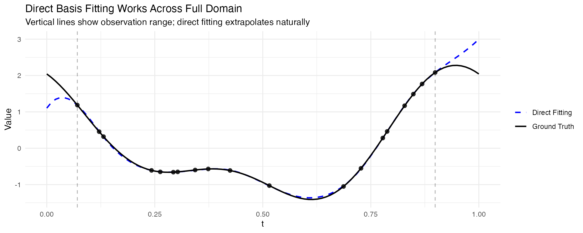

Key observations:

Direct fitting fits basis functions directly to the sparse observations using least squares, and can extrapolate beyond the observed range
Interpolate-then-fit requires observations at domain boundaries; gaps produce NAs
For data with good coverage of the domain, both approaches give similar results
Direct fitting is the safer choice for truly sparse or irregularly sampled data

Alternative: Interpolate Then Fit

For regular data (or after converting irregular to regular), you can use basis projection:

# Simulate regular functional data
set.seed(123)
fd_sim <- simFunData(n = 15, argvals = seq(0, 1, length.out = 100), M = 5, seed = 42)

# Add noise to simulate measurement error
fd_noisy <- fd_sim
fd_noisy$data <- fd_noisy$data + matrix(rnorm(length(fd_noisy$data), sd = 0.3),
                                         nrow = nrow(fd_noisy$data))

# Project onto B-spline basis (smooths the curves)
coefs <- fdata2basis(fd_noisy, nbasis = 12, type = "bspline")
fd_basis <- basis2fdata(coefs, argvals = fd_noisy$argvals)

# Compare using ggplot2
p1 <- autoplot(fd_noisy, alpha = 0.7) + labs(title = "Noisy Data")
p2 <- autoplot(fd_basis, alpha = 0.7) + labs(title = "B-spline Smoothed (12 basis)")
gridExtra::grid.arrange(p1, p2, ncol = 2)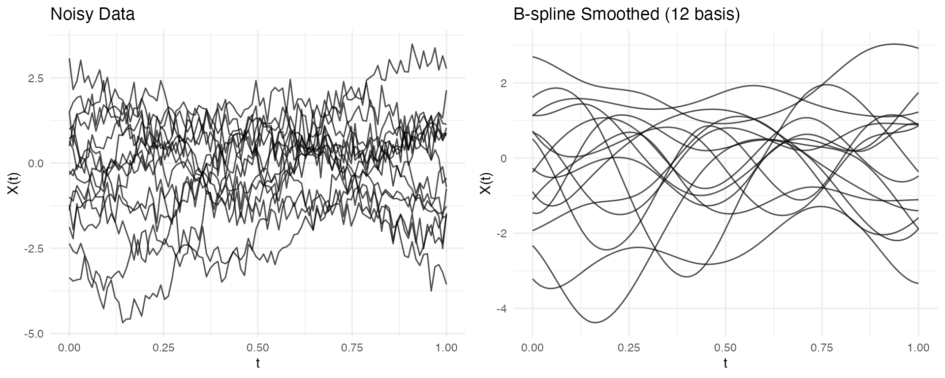

P-spline Smoothing

P-splines with automatic smoothing parameter selection provide robust results for noisy data:

# Create noisy data for P-spline demo
set.seed(456)
fd_for_pspline <- simFunData(n = 15, argvals = seq(0, 1, length.out = 100), M = 5, seed = 42)
fd_for_pspline$data <- fd_for_pspline$data + matrix(rnorm(length(fd_for_pspline$data), sd = 0.3),
                                                      nrow = nrow(fd_for_pspline$data))

# P-spline with fixed lambda (automatic selection can be unstable for some data)
pspline_result <- pspline(fd_for_pspline, nbasis = 20, lambda = 0.01)

# Compare (pspline returns a list; extract $fdata for the smoothed curves)
p1 <- autoplot(fd_for_pspline, alpha = 0.7) + labs(title = "Noisy Data")
p2 <- autoplot(pspline_result$fdata, alpha = 0.7) + labs(title = "P-spline Smoothed")
gridExtra::grid.arrange(p1, p2, ncol = 2)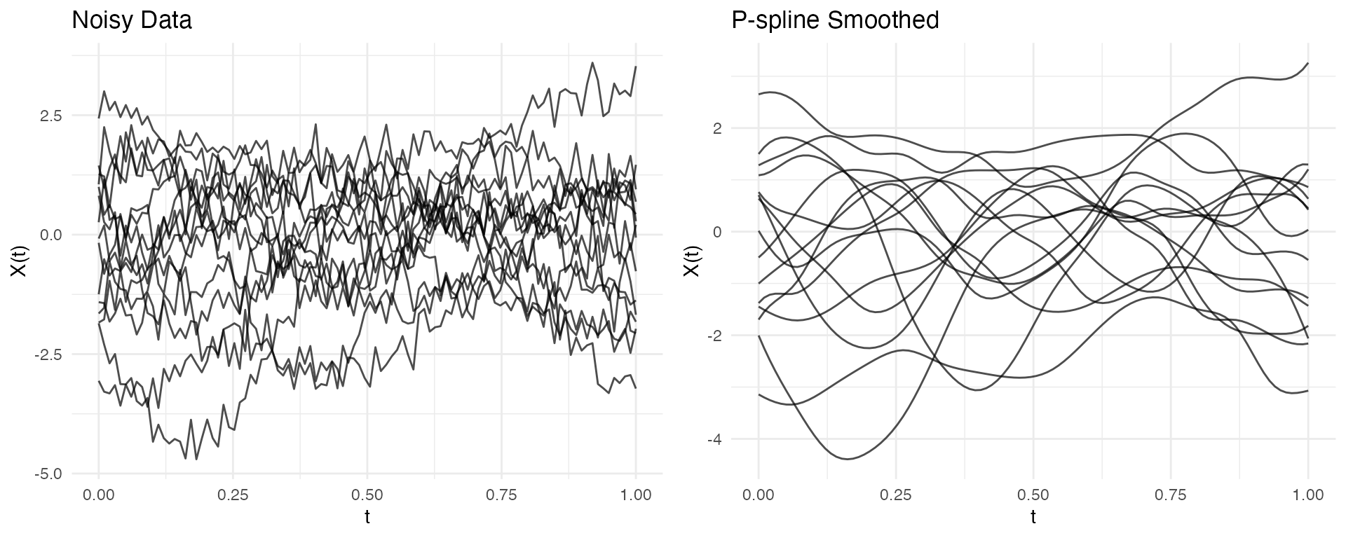

Choosing the Right Approach

Approach	Best For	Key Parameters
Direct basis fitting (irregFdata)	Sparse/irregular data	`nbasis`, `type`
B-spline projection	Regular clean data	`nbasis`, `type="bspline"`
P-spline smoothing	Noisy regular data	`nbasis`, `lambda`
Fourier basis	Periodic/seasonal patterns	`nbasis`, `type="fourier"`

Tip: Use fdata2basis_cv() to automatically select the optimal number of basis functions via cross-validation.

Operations on Irregular Data

Integration

Compute integrals using trapezoidal rule:

# Create data with known integral
argvals <- list(
  seq(0, 1, length.out = 50),
  seq(0, 1, length.out = 30)
)
# Constant function = 1 should integrate to 1
X <- list(rep(1, 50), rep(2, 30))
ifd <- irregFdata(argvals, X)

integrals <- int.simpson(ifd)
print(integrals)  # Should be approximately 1 and 2
#> [1] 1 2

Lp Norms

# L2 norm of constant function c is c
norms <- norm(ifd, p = 2)
print(norms)
#> [1] 1 2

Mean Function Estimation

The mean() function estimates the mean from irregular data. The default method uses basis reconstruction, which preserves the functional structure:

# Simulate many curves
fd <- simFunData(n = 50, argvals = t, M = 5, seed = 42)
ifd <- sparsify(fd, minObs = 15, maxObs = 30, seed = 123)

# Estimate mean (default: basis method)
mean_fd <- mean(ifd)
autoplot(mean_fd) + labs(title = "Estimated Mean Function")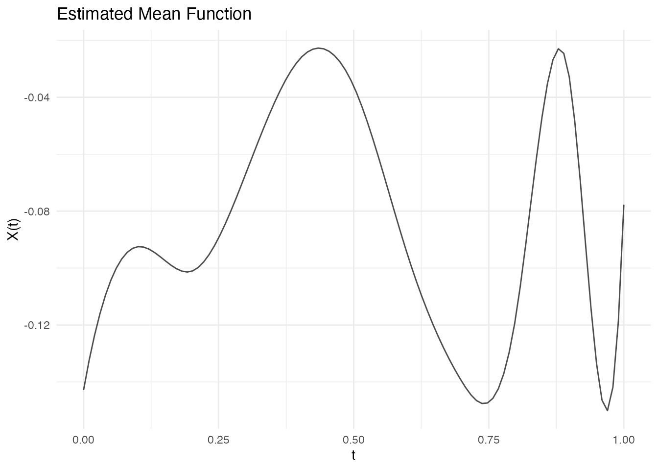

# Compare to true sample mean (from original data)
true_mean <- colMeans(fd$data)

# Also try kernel method for comparison
mean_kernel <- mean(ifd, method = "kernel", bandwidth = 0.1)

# Create comparison data frame
compare_df <- rbind(
  data.frame(t = t, value = true_mean, type = "True Sample Mean"),
  data.frame(t = mean_fd$argvals, value = mean_fd$data[1,], type = "Basis Method"),
  data.frame(t = mean_kernel$argvals, value = mean_kernel$data[1,], type = "Kernel Method")
)

ggplot(compare_df, aes(x = t, y = value, color = type)) +
  geom_line(linewidth = 1) +
  scale_color_manual(values = c("True Sample Mean" = "black",
                                 "Basis Method" = "blue",
                                 "Kernel Method" = "red")) +
  labs(title = "Mean Estimation: Basis vs Kernel",
       subtitle = "Basis method (default) is more accurate",
       x = "t", y = "Mean", color = NULL) +
  theme_minimal()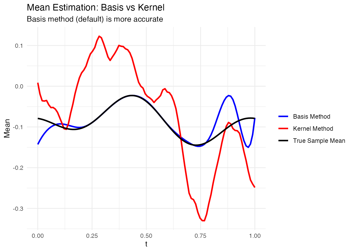

# Compare accuracy
rmse_basis <- sqrt(mean((mean_fd$data[1,] - true_mean)^2))
rmse_kernel <- sqrt(mean((mean_kernel$data[1,] - true_mean)^2))
cat("RMSE (Basis method):", round(rmse_basis, 4), "\n")
#> RMSE (Basis method): 0.0263
cat("RMSE (Kernel method):", round(rmse_kernel, 4), "\n")
#> RMSE (Kernel method): 0.1033

Distance Matrix

Compute pairwise Lp distances:

ifd <- sparsify(fd[1:5], minObs = 20, maxObs = 40, seed = 123)
D <- metric.lp(ifd, p = 2)
round(D, 2)
#>      [,1] [,2] [,3] [,4] [,5]
#> [1,] 0.00 0.69 1.04 1.53 1.32
#> [2,] 0.69 0.00 1.42 1.76 1.57
#> [3,] 1.04 1.42 0.00 1.10 1.47
#> [4,] 1.53 1.76 1.10 0.00 1.04
#> [5,] 1.32 1.57 1.47 1.04 0.00

Subsetting

Extract specific observations:

ifd <- sparsify(fd[1:10], minObs = 10, maxObs = 20, seed = 123)

# Single observation
ifd_sub1 <- ifd[1]
print(ifd_sub1)
#> Irregular Functional Data Object
#> =================================
#>   Number of observations: 1 
#>   Points per curve:
#>     Min: 12 
#>     Median: 12 
#>     Max: 12 
#>     Total: 12 
#>   Domain: [ 0 , 1 ]

# Multiple observations
ifd_sub23 <- ifd[2:3]
print(ifd_sub23)
#> Irregular Functional Data Object
#> =================================
#>   Number of observations: 2 
#>   Points per curve:
#>     Min: 12 
#>     Median: 15.5 
#>     Max: 19 
#>     Total: 31 
#>   Domain: [ 0 , 1 ]

# Negative indexing
ifd_not1 <- ifd[-1]
ifd_not1$n
#> [1] 9

Metadata Support

Store additional covariates with the data:

argvals <- list(c(0, 0.5, 1), c(0, 1), c(0, 0.3, 0.7, 1))
X <- list(c(1, 2, 1), c(0, 2), c(1, 1.5, 1.5, 1))
meta <- data.frame(
  group = c("treatment", "control", "treatment"),
  age = c(45, 52, 38)
)

ifd <- irregFdata(argvals, X,
                  id = c("patient_001", "patient_002", "patient_003"),
                  metadata = meta)

# Access metadata
ifd$id
#> [1] "patient_001" "patient_002" "patient_003"
ifd$metadata
#>       group age
#> 1 treatment  45
#> 2   control  52
#> 3 treatment  38

# Subsetting preserves metadata
ifd[1]$metadata
#>       group age
#> 1 treatment  45

Best Practices

When to Use Irregular Representation

Scenario	Recommendation
Few missing points	Use regular `fdata` with NA
Systematic sparsity	Use `irregFdata`
Very dense data	Use regular `fdata`
Mixed observation times	Use `irregFdata`

Memory Considerations

irregFdata is more memory-efficient when data is sparse:

# Regular: always stores n x m values
n <- 100
m <- 1000
regular_size <- n * m * 8  # bytes (double)

# Irregular: stores only observed values
avg_obs <- 50  # average observations per curve
irreg_size <- n * avg_obs * 8 * 2  # values + argvals

cat("Regular (n=100, m=1000):", regular_size / 1024, "KB\n")
#> Regular (n=100, m=1000): 781.25 KB
cat("Irregular (n=100, ~50 obs each):", irreg_size / 1024, "KB\n")
#> Irregular (n=100, ~50 obs each): 78.125 KB

Preprocessing Recommendations

Quality control: Remove curves with too few observations
Domain alignment: Ensure all curves span similar ranges
Outlier removal: Check for obviously erroneous values
Bandwidth selection: Use cross-validation for kernel smoothing

# Remove curves with fewer than 5 observations
min_obs <- 5
keep <- sapply(ifd$X, length) >= min_obs

if (any(!keep)) {
  ifd_clean <- ifd[keep]
  cat("Removed", sum(!keep), "curves with <", min_obs, "observations\n")
}
#> Removed 3 curves with < 5 observations

Summary

Function	Purpose
`irregFdata()`	Create irregular functional data objects
`is.irregular()`	Check if object is irregFdata
`sparsify()`	Convert regular to irregular data
`as.fdata()`	Convert irregular to regular (with interpolation)
`fdata2basis()`	Fit basis coefficients (works with fdata and irregFdata)
`basis2fdata()`	Reconstruct curves from coefficients
`int.simpson()`	Compute integrals (works with fdata and irregFdata)
`norm()`	Compute Lp norms (works with fdata and irregFdata)
`mean()`	Estimate mean via kernel smoothing
`metric.lp()`	Compute pairwise distances (works with fdata and irregFdata)