Visualize functional principal component analysis results with multiple plot types: component perturbation plots, variance explained (scree plot), or score plots.
Arguments
- x
An object of class 'fdata2pc' from
fdata2pc.- type
Type of plot: "components" (default) shows mean +/- scaled PC loadings, "variance" shows a scree plot of variance explained, "scores" shows PC1 vs PC2 scatter plot of observations.
- ncomp
Number of components to display (default 3 or fewer if not available).
- multiple
Factor for scaling PC perturbations. Default is 2 (shows +/- 2*sqrt(eigenvalue)*PC).
- show_both_directions
Logical. If TRUE (default), show both positive and negative perturbations (mean + PC and mean - PC). If FALSE, only show positive perturbation. All curves are solid lines differentiated by color.
- ...
Additional arguments passed to plotting functions.
Details
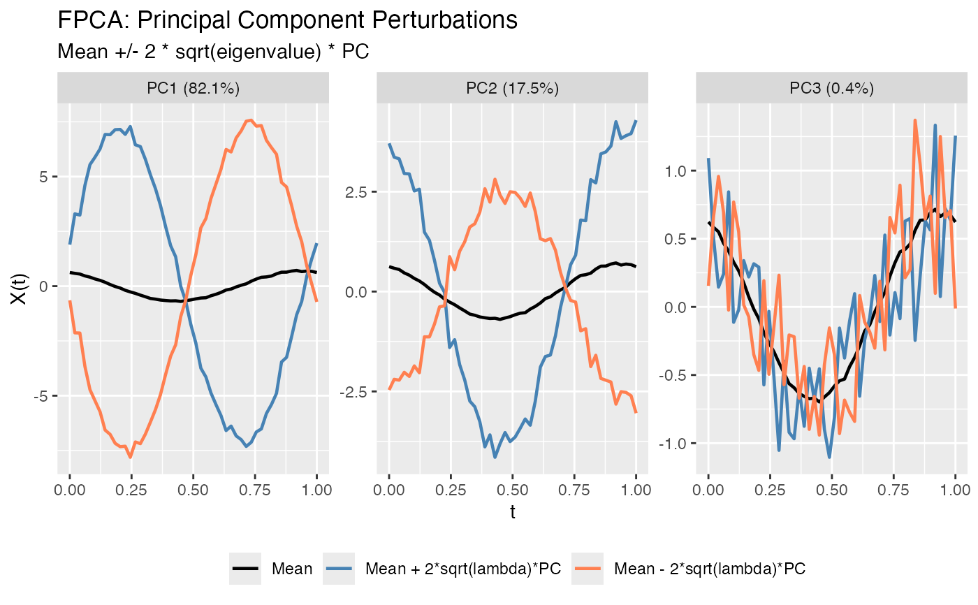
The "components" plot shows the mean function (black) with perturbations in the direction of each principal component. The perturbation is computed as: mean +/- multiple * sqrt(variance_explained) * PC_loading. All lines are solid and differentiated by color only.
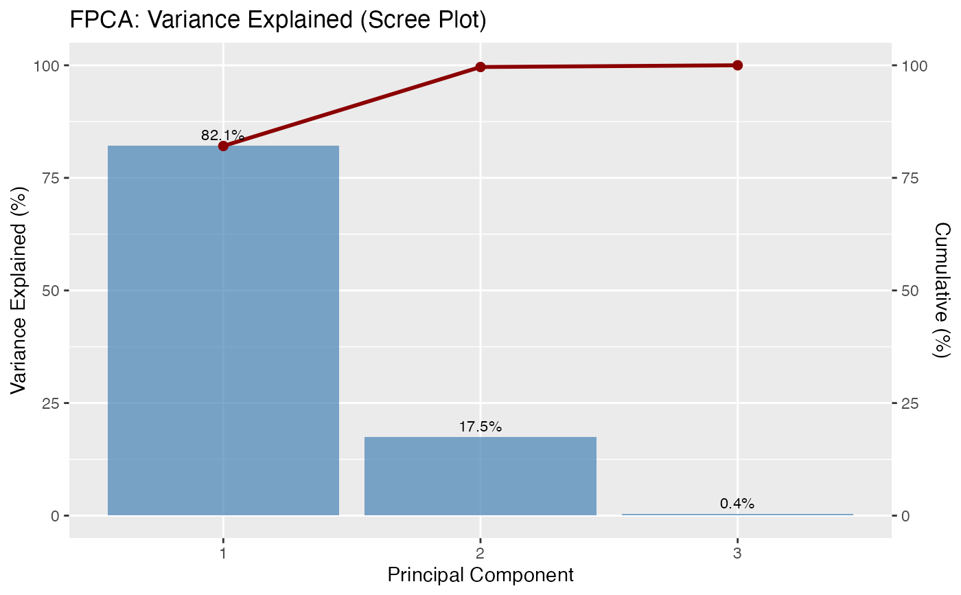
The "variance" plot shows a scree plot with the proportion of variance explained by each component as a bar chart.
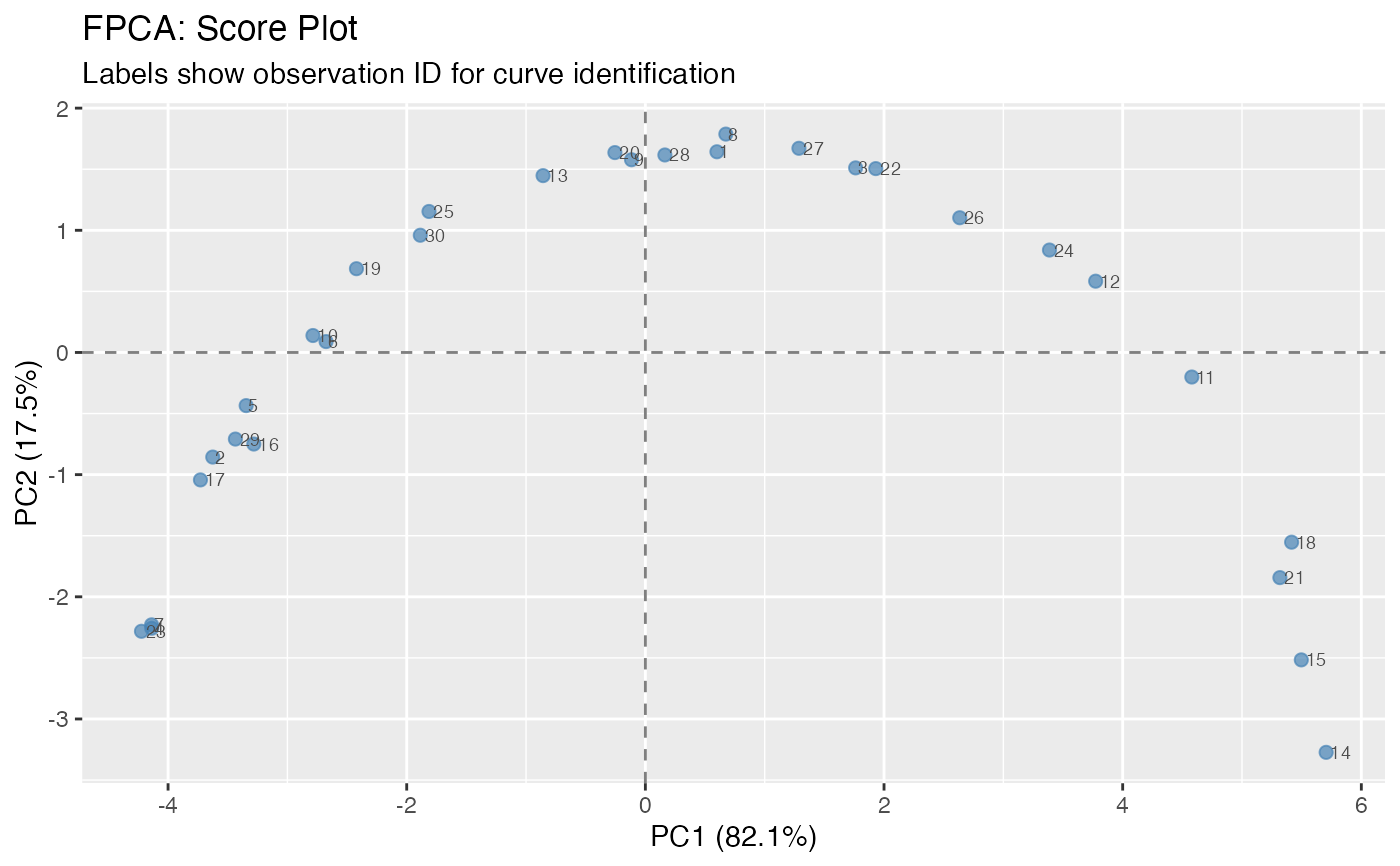
The "scores" plot shows a scatter plot of observations in PC space, typically PC1 vs PC2.
See also
fdata2pc for computing FPCA.
Examples
t <- seq(0, 1, length.out = 50)
X <- matrix(0, 30, 50)
for (i in 1:30) X[i, ] <- sin(2*pi*t + runif(1, 0, pi)) + rnorm(50, sd = 0.1)
fd <- fdata(X, argvals = t)
pc <- fdata2pc(fd, ncomp = 3)
# Plot PC components (mean +/- perturbations)
plot(pc, type = "components")
 # Scree plot
plot(pc, type = "variance")
# Scree plot
plot(pc, type = "variance")
 # Score plot
plot(pc, type = "scores")
# Score plot
plot(pc, type = "scores")