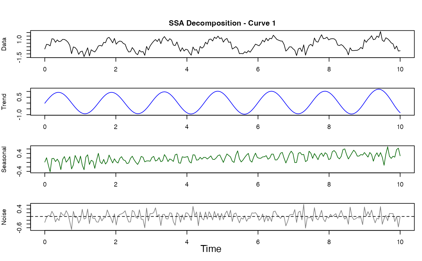
Singular Spectrum Analysis (SSA) for Time Series Decomposition

Performs Singular Spectrum Analysis on functional data to decompose each curve into trend, seasonal (oscillatory), and noise components. SSA is a model-free, non-parametric technique based on singular value decomposition of the trajectory matrix.

Usage

ssa.fd(fdataobj, window.length = NULL, n.components = 10)

Arguments

fdataobj: An fdata object.
window.length: Embedding window length (L). If NULL, automatically determined as min(n/2, 50). Larger values capture longer-term patterns.
n.components: Number of SVD components to extract. Default: 10. More components allow finer decomposition but increase noise.

Value

A list of class "ssa_result" with components:

trend: fdata object containing reconstructed trend component
seasonal: fdata object containing reconstructed seasonal component
noise: fdata object containing noise/residual component
singular.values: Singular values from SVD (sorted descending)
contributions: Proportion of variance explained by each component
window.length: Window length used
n.components: Number of components extracted
detected.period: Auto-detected period (if any)
confidence: Confidence score for detected period
call: The function call

Details

The SSA algorithm consists of four stages:

1. Embedding: The time series is converted into a trajectory matrix by arranging lagged versions of the series as columns.

2. SVD Decomposition: Singular value decomposition of the trajectory matrix produces orthogonal components.

3. Grouping: Components are grouped into trend (slowly varying), seasonal (oscillatory), and noise. Auto-detection uses sign change analysis and autocorrelation.

4. Reconstruction: Diagonal averaging (Hankelization) converts grouped trajectory matrices back to time series.

SSA is particularly suited for:

Short time series where spectral methods fail
Noisy data with weak periodic signals
Non-stationary data with changing trend
Separating multiple periodicities

References

Golyandina, N., & Zhigljavsky, A. (2013). Singular Spectrum Analysis for Time Series. Springer.

Elsner, J. B., & Tsonis, A. A. (1996). Singular Spectrum Analysis: A New Tool in Time Series Analysis. Plenum Press.

Examples

# Signal with trend + seasonal + noise
t <- seq(0, 10, length.out = 200)
X <- matrix(0.05 * t + sin(2 * pi * t / 1.5) + rnorm(length(t), sd = 0.3), nrow = 1)
fd <- fdata(X, argvals = t)

# Perform SSA
result <- ssa.fd(fd)
print(result)
#> Singular Spectrum Analysis (SSA)
#> --------------------------------
#> Window length:    50
#> N components:     10
#> Detected period:  2.00
#> Confidence:       0.4804
#> 
#> Number of curves: 1
#> Series length:    200
#> 
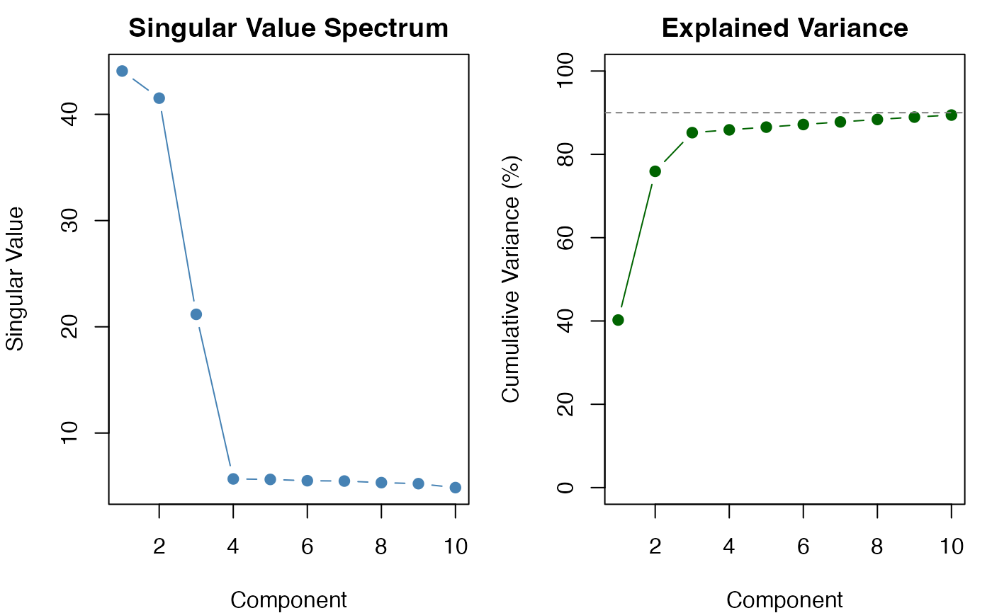
#> Top component contributions:
#>   Component 1: 40.2%
#>   Component 2: 35.7%
#>   Component 3: 9.3%
#>   Component 4: 0.7%
#>   Component 5: 0.7%
#>   Cumulative:   86.5%
#> 
#> Variance decomposition:
#>   Trend:    83.6%
#>   Seasonal: 6.0%
#>   Noise:    10.5%

# Plot components
plot(result)


# Examine singular value spectrum (scree plot)
plot(result, type = "spectrum")