Simulate Functional Data via Karhunen-Loeve Expansion

Generates functional data samples using a truncated Karhunen-Loeve representation: f_i(t) = mean(t) + sum_{k=1}^M xi_{ik} * phi_k(t) where xi_{ik} ~ N(0, lambda_k).

Usage

simFunData(
  n,
  argvals,
  M,
  eFun.type = c("Fourier", "Poly", "PolyHigh", "Wiener"),
  eVal.type = c("linear", "exponential", "wiener"),
  mean = NULL,
  seed = NULL
)

Arguments

n

Number of curves to generate.

argvals

Numeric vector of evaluation points.

M

Number of basis functions (eigenfunctions) to use.

eFun.type

Type of eigenfunction basis: "Fourier", "Poly", "PolyHigh", or "Wiener".

eVal.type

Type of eigenvalue decay: "linear", "exponential", or "wiener".

mean

Mean function. Can be:

• NULL for zero mean

• A numeric vector of length equal to argvals

• A function that takes argvals as input

seed

Optional integer random seed for reproducibility.

Value

An fdata object containing the simulated functional data.

Details

The Karhunen-Loeve expansion provides a natural way to simulate Gaussian functional data with a specified covariance structure. The eigenvalues control the variance contribution of each mode, while the eigenfunctions determine the shape of variation.

The theoretical covariance function is: Cov(X(s), X(t)) = sum_{k=1}^M lambda_k * phi_k(s) * phi_k(t)

See also

eFun, eVal, addError, make.gaussian.process

Examples

t <- seq(0, 1, length.out = 100)

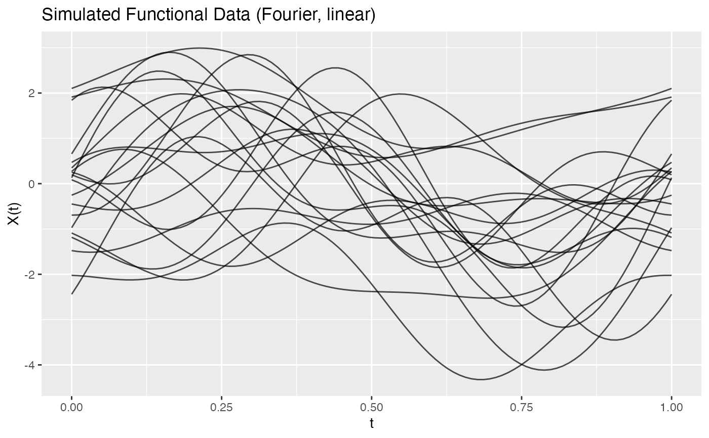
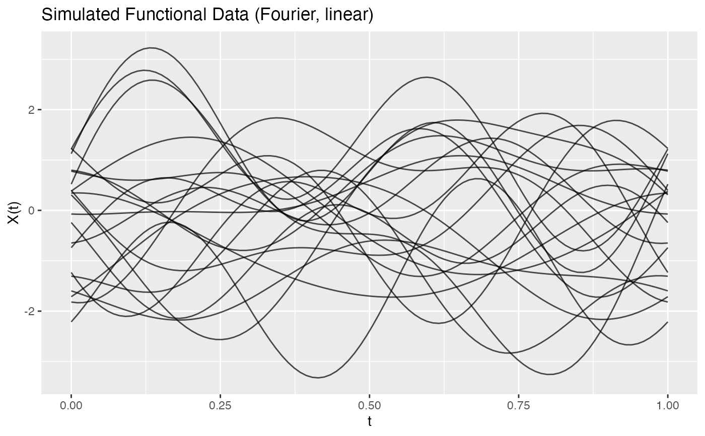
# Basic simulation with Fourier basis
fd <- simFunData(n = 20, argvals = t, M = 5,
                 eFun.type = "Fourier", eVal.type = "linear")
plot(fd, main = "Simulated Functional Data (Fourier, Linear)")


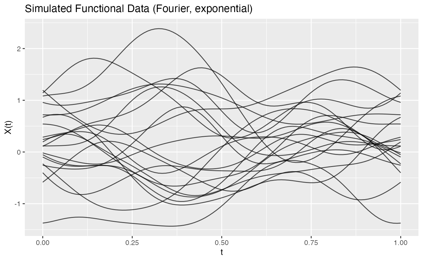
# Smoother curves with exponential decay
fd_smooth <- simFunData(n = 20, argvals = t, M = 10,
                        eFun.type = "Fourier", eVal.type = "exponential")
plot(fd_smooth, main = "Smooth Simulated Data (Exponential Decay)")


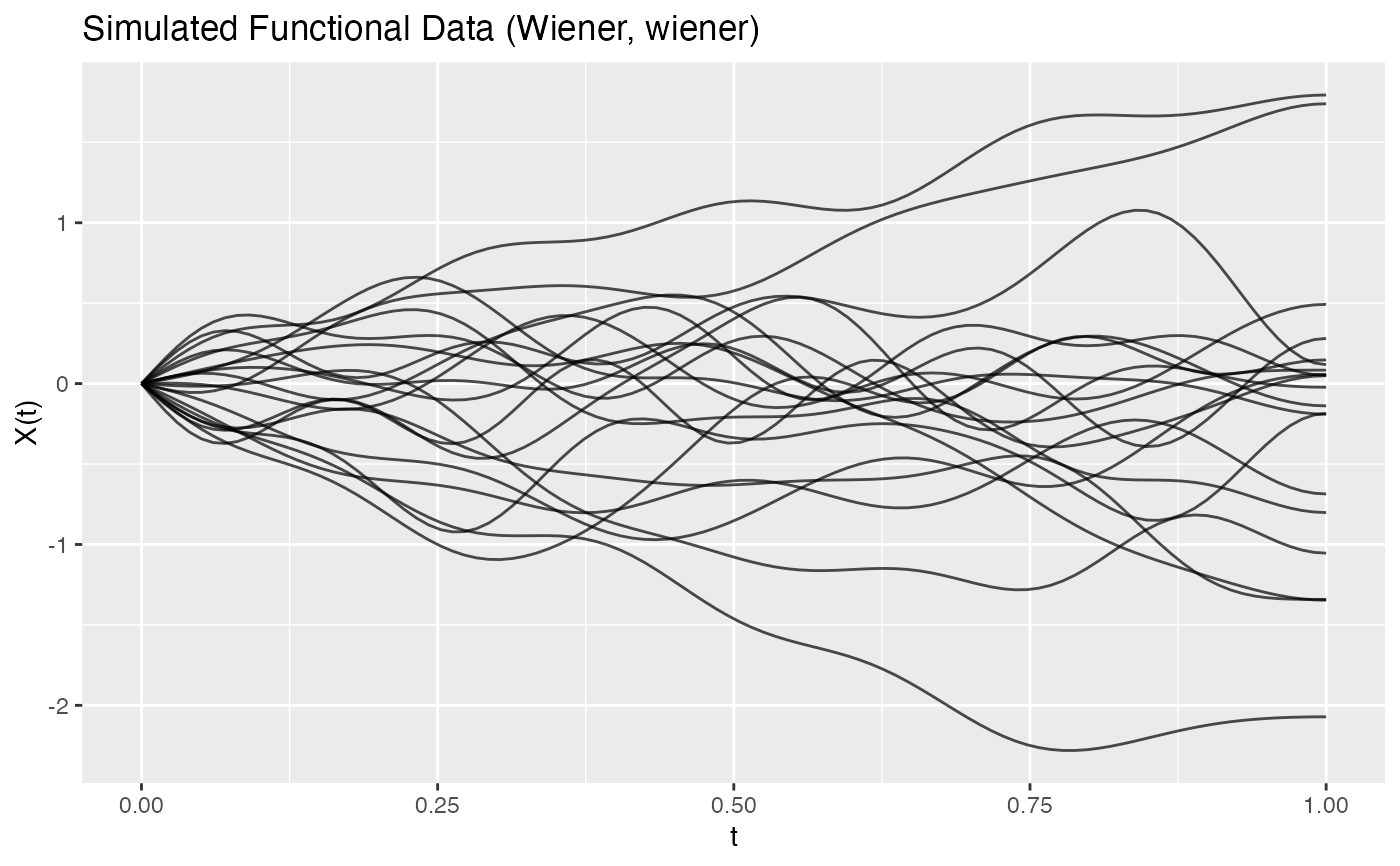
# Wiener process simulation
fd_wiener <- simFunData(n = 20, argvals = t, M = 10,
                        eFun.type = "Wiener", eVal.type = "wiener", seed = 42)
plot(fd_wiener, main = "Wiener Process Simulation")


# With mean function
mean_fn <- function(t) sin(2 * pi * t)
fd_mean <- simFunData(n = 20, argvals = t, M = 5, mean = mean_fn, seed = 42)
plot(fd_mean, main = "Simulated Data with Sinusoidal Mean")