Equivalence Testing¶

Classical hypothesis tests ask "are these two groups different?" Equivalence testing flips the question: are these two groups similar enough to be considered practically the same?

This is critical in manufacturing (batch-to-batch consistency), bioequivalence studies (generic vs. brand-name drugs), and any domain where you need to demonstrate that a change or substitution has no meaningful effect on the functional response.

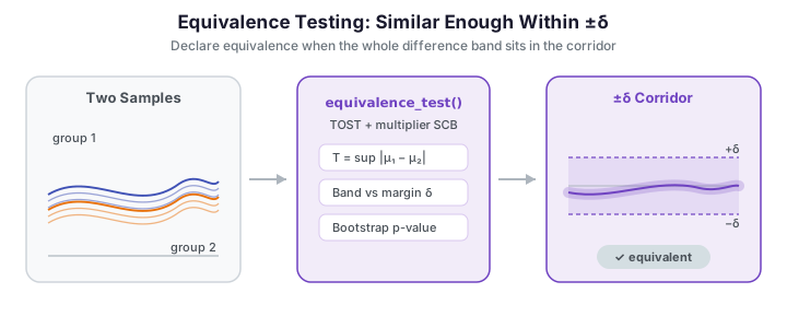
The TOST framework¶

The functional equivalence test in fdars implements a Two One-Sided Tests (TOST) procedure adapted for functional data:

Define an equivalence margin \(\delta > 0\).
Test \(H_0^-: \|\mu_1 - \mu_2\|_\infty \ge \delta\) against \(H_1^-: \|\mu_1 - \mu_2\|_\infty < \delta\).
If \(H_0^-\) is rejected at level \(\alpha\), the two groups are declared equivalent within margin \(\delta\).

The null distribution of the test statistic is estimated via a Gaussian multiplier bootstrap.

\[ T = \sup_{t \in \mathcal{T}} \left| \bar X_1(t) - \bar X_2(t) \right| \]

Equivalence is concluded when \(T < \delta - c_\alpha\), where \(c_\alpha\) is the \((1-\alpha)\) quantile from the bootstrap.

Usage¶

import numpy as np
from fdars import Fdata
from fdars.simulation import simulate
from fdars.tolerance import equivalence_test

argvals = np.linspace(0, 1, 100)

# Two groups with very similar means
fd_a = Fdata(simulate(50, argvals, n_basis=5, seed=1), argvals=argvals)
fd_b = Fdata(simulate(50, argvals, n_basis=5, seed=2) + 0.2, argvals=argvals)  # small offset

result = equivalence_test(
    data1=fd_a.data,
    data2=fd_b.data,
    delta=1.0,       # equivalence margin
    alpha=0.05,      # significance level
    nb=1000,         # bootstrap replicates
    seed=42,
)

Parameters

Parameter	Type	Default	Description
`data1`	`ndarray (n1, m)`	--	First group of functional observations
`data2`	`ndarray (n2, m)`	--	Second group of functional observations
`delta`	`float`	--	Equivalence margin (\(\delta > 0\))
`alpha`	`float`	`0.05`	Significance level
`nb`	`int`	`1000`	Number of bootstrap replicates
`seed`	`int`	`42`	Random seed

Returns a dictionary:

Key	Type	Description
`equivalent`	`bool`	`True` if equivalence is established at level \(\alpha\)
`p_value`	`float`	Bootstrap p-value
`test_statistic`	`float`	Observed sup-norm of the mean difference

print(f"Equivalent: {result['equivalent']}")
print(f"p-value:    {result['p_value']:.4f}")
print(f"Sup-norm:   {result['test_statistic']:.4f}")

Choosing the margin \(\delta\)¶

The margin \(\delta\) is the maximum allowable pointwise difference between the two mean functions. It should be set before looking at the data, based on domain knowledge:

Do not choose \(\delta\) from the data

Setting \(\delta\) to be just larger than the observed difference inflates the Type I error. Always specify \(\delta\) based on what constitutes a practically meaningful difference in your application.

Domain	Typical \(\delta\) guidance
Manufacturing	Specification tolerance / 2
Bioequivalence	20 % of the reference mean (FDA guidance)
Environmental monitoring	Regulatory action threshold

Example -- equivalent vs. non-equivalent groups¶

import numpy as np
from fdars import Fdata
from fdars.simulation import simulate
from fdars.tolerance import equivalence_test

argvals = np.linspace(0, 1, 100)
delta = 1.0

# ── Case 1: Similar groups (should be equivalent) ────────────
fd_a = Fdata(simulate(40, argvals, n_basis=5, seed=10), argvals=argvals)
fd_b = Fdata(simulate(40, argvals, n_basis=5, seed=20) + 0.1, argvals=argvals)

r1 = equivalence_test(fd_a.data, fd_b.data, delta=delta, alpha=0.05, nb=2000, seed=42)
print(f"Case 1 — Equivalent: {r1['equivalent']}  p={r1['p_value']:.4f}")

# ── Case 2: Different groups (should NOT be equivalent) ──────
fd_c = Fdata(simulate(40, argvals, n_basis=5, seed=10), argvals=argvals)
fd_d = Fdata(simulate(40, argvals, n_basis=5, seed=20) + 5.0, argvals=argvals)  # large shift

r2 = equivalence_test(fd_c.data, fd_d.data, delta=delta, alpha=0.05, nb=2000, seed=42)
print(f"Case 2 — Equivalent: {r2['equivalent']}  p={r2['p_value']:.4f}")

Expected output:

Case 1 — Equivalent: True   p=0.00..
Case 2 — Equivalent: False  p=1.00..

Sensitivity to \(\delta\)¶

You can sweep over a range of margins to understand how sensitive the conclusion is:

import numpy as np
from fdars import Fdata
from fdars.simulation import simulate
from fdars.tolerance import equivalence_test

argvals = np.linspace(0, 1, 100)
fd_a = Fdata(simulate(50, argvals, n_basis=5, seed=1), argvals=argvals)
fd_b = Fdata(simulate(50, argvals, n_basis=5, seed=2) + 0.3, argvals=argvals)

for delta in [0.2, 0.5, 1.0, 2.0, 5.0]:
    r = equivalence_test(fd_a.data, fd_b.data, delta=delta, nb=1000, seed=42)
    status = "equivalent" if r["equivalent"] else "not equivalent"
    print(f"delta={delta:.1f}  T={r['test_statistic']:.3f}  p={r['p_value']:.3f}  -> {status}")

References

- Dette, H., Kokot, K. (2021). Detecting relevant differences in the covariance operators of functional time series. Biometrika, 108(4), 895–913.
- Wellek, S. (2010). Testing Statistical Hypotheses of Equivalence and Noninferiority, 2nd ed. Chapman & Hall/CRC.
- Degras, D.A. (2011). Simultaneous confidence bands for nonparametric regression with functional data. Statistica Sinica, 21(4), 1735–1765.