Classification

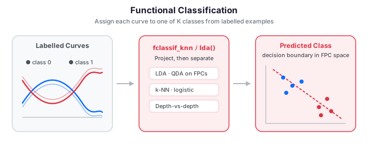
Functional classification assigns a class label \(g_i \in \{0, 1, \dots, K-1\}\) to each functional observation \(x_i(t)\). Two things make this harder than ordinary classification:

• Curse of dimensionality. With \(m\) grid points (often 100–1000), standard classifiers break down when \(n \ll m\): covariance matrices become singular and decision boundaries overfit.
• Ignoring smoothness. Treating \(x_i(t_1)\) and \(x_i(t_2)\) as unrelated features discards the continuity that makes the data functional.

fdars resolves this by projecting curves onto a low-dimensional FPC basis and classifying in that reduced space (LDA, QDA, k-NN, logistic), or by working directly in function space with a proper functional distance or depth (kernel, depth-vs-depth). All of these are available, plus cross-validated model comparison.

Classification exploits differences in the class-mean curves. Below, two classes are separated by a phase difference (a sine vs. a cosine); the bold curves are the per-class mean functions the classifiers learn to distinguish.

The two bold class-mean curves are cleanly offset — a sine against a cosine — so even though individual noisy realisations overlap, LDA reaches near-perfect accuracy by projecting onto the FPC directions that capture this mean difference.

---

Discriminant analysis

Both discriminant methods work on the FPC scores \(\xi_i \in \mathbb{R}^K\) and model each class as Gaussian in that space.

LDA (Linear Discriminant Analysis)

LDA assumes a shared covariance \(\Sigma\) across classes. Each observation is assigned to the class maximising the log-posterior discriminant

\[ \delta_g(\xi) = \log \pi_g - \tfrac12 (\xi - \mu_g)^\top \Sigma^{-1} (\xi - \mu_g), \]

which produces linear decision boundaries.

import numpy as np
from fdars import Fdata
from fdars.classification import fclassif_lda

# --- Simulate two-class functional data ---
np.random.seed(0)
n, m = 80, 101
t = np.linspace(0, 1, m)

raw = np.zeros((n, m))
labels = np.zeros(n, dtype=np.int64)
for i in range(n):
    if i < n // 2:
        raw[i] = np.sin(2 * np.pi * t) + 0.3 * np.random.randn(m)
        labels[i] = 0
    else:
        raw[i] = np.cos(2 * np.pi * t) + 0.3 * np.random.randn(m)
        labels[i] = 1
fd = Fdata(raw, argvals=t)

result = fclassif_lda(fd.data, labels, ncomp=3)
print(f"LDA accuracy: {result['accuracy']:.2%}")
print(f"Predictions:  {result['predicted'][:10]}")

Key	Type	Description
predicted	ndarray (n,)	Predicted class labels
accuracy	float	Resubstitution accuracy

QDA (Quadratic Discriminant Analysis)

QDA relaxes the shared-covariance assumption, estimating a separate \(\Sigma_g\) per class. The extra \(-\tfrac12\log|\Sigma_g|\) term makes the boundaries quadratic (ellipsoidal), at the cost of needing more observations per class.

from fdars.classification import fclassif_qda

result = fclassif_qda(fd.data, labels, ncomp=3)
print(f"QDA accuracy: {result['accuracy']:.2%}")

LDA vs. QDA

Use LDA when classes share similar covariance structure and sample sizes are small. Use QDA when class covariances differ substantially and you have enough observations per class (\(n_g > K(K+1)/2\)).

---

k-Nearest Neighbors

k-NN makes no distributional assumption. It classifies each observation by a majority vote among its \(k\) nearest neighbours in FPC score space, using the Euclidean distance \(\lVert \xi_i - \xi_j \rVert_2\).

from fdars.classification import fclassif_knn

result = fclassif_knn(fd.data, labels, ncomp=3, k=5)
print(f"k-NN accuracy (k=5): {result['accuracy']:.2%}")

Small \(k\) gives a flexible but noisy boundary; large \(k\) gives a smooth but possibly biased one. Choose \(k\) (and ncomp) by cross-validation.

---

Kernel classifier

A fully nonparametric classifier that operates directly on the curves via an \(L^2\) functional distance, skipping the FPC projection. For a query curve \(X\) it sums Gaussian kernel weights \(K(d, h) = \exp(-d^2/2h^2)\) over each class and picks the class with the largest total weight:

\[ \hat g(X) = \arg\max_g \sum_{j:\,y_j = g} K\big(d(X, X_j), h\big). \]

from fdars.classification import fclassif_kernel

result = fclassif_kernel(fd.data, fd.argvals, labels, h_func=1.0, h_scalar=1.0)
print(f"Kernel accuracy: {result['accuracy']:.2%}")

Parameter	Description
h_func	Bandwidth for the functional distance kernel
h_scalar	Bandwidth for the scalar kernel

---

Depth-vs-depth classifier

The DD-classifier computes the statistical depth of each curve with respect to each class distribution — no dimension reduction, no explicit distances. Using an integrated depth \(D_g(X) = \int_0^1 D_1(X(t); F_{g,t})\,dt\), each curve maps to the point \((D_1(X), \dots, D_K(X))\) in depth space, and is assigned to the class where it is most central. Because depth is rank-based, this classifier is robust to outliers.

from fdars.classification import fclassif_dd

result = fclassif_dd(fd.data, labels)
print(f"DD-classifier accuracy: {result['accuracy']:.2%}")

It returns predicted and accuracy, like the discriminant methods, but takes no ncomp — depth is computed on the raw curves.

---

Cross-validated classification

Resubstitution accuracy is optimistic. fclassif_cv estimates the out-of-sample error by \(k\)-fold cross-validation and simultaneously searches component counts from 1 to ncomp, reporting the best_ncomp.

from fdars.classification import fclassif_cv

# Compare methods
for method in ["lda", "qda", "knn"]:
    result = fclassif_cv(
        fd.data, fd.argvals, labels,
        method=method,
        ncomp=5,
        nfold=5,
    )
    print(f"{method.upper():>6s}: error rate = {result['error_rate']:.2%}, "
          f"best_ncomp = {result['best_ncomp']}")

Key	Type	Description
error_rate	float	Cross-validated error rate
fold_errors	ndarray (nfold,)	Error rate for each fold
best_ncomp	int	Optimal number of components

Validation — CV accuracy beats chance, and out-of-sample ≥ in-sample error

Two ground-truth checks on a fresh two-class problem: (1) the cross-validated accuracy must clear the \(1/K\) chance rate by a clear margin, and (2) the honest out-of-sample (CV) error must be at least the optimistic resubstitution error — a property that always holds in expectation. Both assertions run below and pass.

import numpy as np
from fdars.classification import fclassif_lda, fclassif_cv

np.random.seed(11)
n, m = 120, 101
t = np.linspace(0, 1, m)
raw = np.zeros((n, m))
labels = np.zeros(n, dtype=np.int64)
for i in range(n):
    if i < n // 2:
        raw[i] = np.sin(2 * np.pi * t) + 0.3 * np.random.randn(m)
    else:
        raw[i] = np.cos(2 * np.pi * t) + 0.3 * np.random.randn(m)
        labels[i] = 1

n_classes = 2
chance = 1.0 / n_classes                       # 0.5 for a balanced 2-class problem

cv = fclassif_cv(raw, t, labels, method="lda", ncomp=5, nfold=5)
cv_accuracy = 1.0 - cv["error_rate"]
insample_error = 1.0 - fclassif_lda(raw, labels, ncomp=cv["best_ncomp"])["accuracy"]

print(f"chance accuracy      = {chance:.2f}")
print(f"CV accuracy          = {cv_accuracy:.3f}")
print(f"in-sample error      = {insample_error:.3f}")
print(f"CV (out-of-sample)   = {cv['error_rate']:.3f}")

# (1) CV accuracy clears chance by a solid margin.
assert cv_accuracy > chance + 0.20, cv_accuracy
# (2) Honest CV error is not optimistic relative to resubstitution.
assert cv["error_rate"] >= insample_error - 1e-9, (cv["error_rate"], insample_error)
print("validation OK: CV accuracy > chance, and OOF error >= in-sample error")

chance accuracy = 0.50 CV accuracy = 1.000 in-sample error = 0.000 CV (out-of-sample) = 0.000 validation OK: CV accuracy > chance, and OOF error >= in-sample error

The separable two-class signal drives CV accuracy well above 0.5, and the cross-validated error never dips below the resubstitution error — the expected ordering between optimistic and honest estimates.

Choosing the number of components

Early FPC components capture the dominant modes of between-class variation and improve discrimination; later components bring in mostly within-class noise and dilute the signal. Plotting CV error against ncomp shows the sweet spot.

import numpy as np
from docs_fig import fig, render
from fdars.classification import fclassif_cv

np.random.seed(4)
n, m = 36, 101
t = np.linspace(0, 1, m)
s1, c1 = np.sin(2 * np.pi * t), np.cos(2 * np.pi * t)
s2, c2 = np.sin(4 * np.pi * t), np.cos(4 * np.pi * t)
s3 = np.sin(6 * np.pi * t)
raw = np.zeros((n, m))
labels = np.zeros(n, dtype=np.int64)
for i in range(n):
    c = i % 2
    labels[i] = c
    # The class signal lives in the first two FPC directions but OVERLAPS the
    # within-class spread there (so it is not trivially separable); modes 3+ are
    # pure within-class noise. With a small sample, including those later
    # components degrades the pooled-covariance estimate and hurts LDA.
    mu = (0.8 * s1 + 0.6 * c1) if c else 0.0 * s1
    raw[i] = mu + 0.5 * np.random.randn() * s1 + 0.5 * np.random.randn() * c1
    raw[i] += (0.3 * np.random.randn() * s2 + 0.25 * np.random.randn() * c2
               + 0.2 * np.random.randn() * s3)
    raw[i] += 0.15 * np.random.randn(m)

ks = range(1, 8)
errs = [fclassif_cv(raw, t, labels, method="lda", ncomp=k, nfold=6)["error_rate"]
        for k in ks]

f, ax = fig()
ax.plot(list(ks), errs, "-o", color="#3f51b5")
ax.set(title="LDA component selection", xlabel="number of FPC components",
       ylabel="10-fold CV error rate")
print(render(f))

The CV error dips to a minimum at a small component count and then climbs again as later, noise-dominated modes enter the pooled covariance — the classic under-fit/over-fit valley that tells you exactly how many FPC directions to keep.

Now add a figure showing the logistic model's calibrated output. Because functional_logistic returns per-curve probabilities \(P(G=1\mid x)\), we can plot them against the FPC-1 score to see the sigmoid boundary the model learns:

import numpy as np
from docs_fig import fig, render
from fdars.regression import fpca, functional_logistic

np.random.seed(7)
n, m = 100, 101
t = np.linspace(0, 1, m)
raw = np.zeros((n, m))
labels = np.zeros(n, dtype=np.int64)
for i in range(n):
    if i < n // 2:
        raw[i] = np.sin(2 * np.pi * t) + 0.4 * np.random.randn(m)
    else:
        raw[i] = np.cos(2 * np.pi * t) + 0.4 * np.random.randn(m)
        labels[i] = 1

score1 = np.asarray(fpca(raw, t, n_comp=1)["scores"])[:, 0]
res = functional_logistic(raw, labels.astype(np.float64), n_comp=3)
probs = np.asarray(res["probabilities"])

f, ax = fig()
order = np.argsort(score1)
ax.plot(score1[order], probs[order], color="#6c757d", lw=1.2, alpha=0.7)
for cls, color, name in [(0, "#3f51b5", "class 0"), (1, "#e8710a", "class 1")]:
    sel = labels == cls
    ax.scatter(score1[sel], probs[sel], color=color, s=30, alpha=0.8, label=name)
ax.axhline(0.5, color="#dc3545", ls="--", lw=1, label="decision threshold")
ax.set(title="Logistic probabilities vs. leading FPC score",
       xlabel="FPC-1 score", ylabel=r"$P(G=1\mid x)$", ylim=(-0.05, 1.05))
ax.legend(fontsize=8)
print(render(f))

The probability curve sweeps smoothly from 0 to 1 as the FPC-1 score grows, with the two classes separating on either side of the 0.5 threshold — points stranded near 0.5 are precisely the ambiguous curves in the overlap region.

---

Functional logistic regression

For binary classification, functional logistic regression models the log-odds as a linear functional of the predictor:

\[ \log\frac{P(G=1 \mid x)}{P(G=0 \mid x)} = \alpha + \int_{\mathcal{T}} x(t)\,\beta(t)\,dt. \]

After the FPC reduction this becomes \(\alpha + \sum_k \gamma_k \xi_{ik}\), fitted by iteratively reweighted least squares (IRLS). Unlike the discriminant methods, it returns calibrated probabilities \(P(G=1\mid x)\), useful for risk scoring and threshold tuning.

from fdars.regression import functional_logistic

result = functional_logistic(fd.data, labels.astype(np.float64), n_comp=3)

probs     = result["probabilities"]       # (n,) -- P(G=1 | x)
predicted = result["predicted_classes"]   # (n,)
beta_t    = result["beta_t"]              # (m,) -- coefficient function
intercept = result["intercept"]           # scalar
coefs     = result["coefficients"]        # FPC coefficients

accuracy = np.mean(predicted == labels)
print(f"Logistic accuracy: {accuracy:.2%}")
print(f"Intercept: {intercept:.4f}")

Key	Type	Description
probabilities	ndarray (n,)	Predicted probabilities for class 1
predicted_classes	ndarray (n,)	Predicted labels
beta_t	ndarray (m,)	Coefficient function \(\hat{\beta}(t)\)
intercept	float	Intercept \(\hat{\alpha}\)
coefficients	ndarray (k,)	Coefficients on FPC scores

Probabilities near 0 or 1 indicate confident classifications; values near 0.5 mark curves in the overlap region.

Phase-invariant logistic regression

When classes differ in the timing of features rather than their amplitude, functional_logistic on raw curves can struggle. The elastic regression page covers elastic_logistic, which aligns curves and classifies in the phase-invariant SRSF domain.

---

Real data: separating two phonemes

The phoneme dataset contains log-periodograms for five spoken sounds. The pair aa (as in dark) and ao (as in water) is the classic hard case — their spectra overlap heavily in the low frequencies. Here we build a binary problem from those two classes and compare classifiers with cross-validation.

import numpy as np
from docs_fig import fig, render
from docs_data import load_phoneme
from fdars.classification import fclassif_cv, fclassif_lda

freq, X, meta = load_phoneme()
ph = meta["phoneme"].to_numpy()
mask = np.isin(ph, ["aa", "ao"])
Xb = X[mask]
yb = (ph[mask] == "ao").astype(np.int64)

# Cross-validated error for three classifiers
scores = {}
for method in ["lda", "qda", "knn"]:
    scores[method] = fclassif_cv(Xb, freq, yb, method=method,
                                 ncomp=6, nfold=5)["error_rate"]

# Class-mean spectra
f, ax = fig()
for cls, color, name in [(0, "#3f51b5", "aa"), (1, "#e8710a", "ao")]:
    ax.plot(freq, Xb[yb == cls].mean(0), color=color, lw=2.4, label=f"{name} mean")
    ax.plot(freq, Xb[yb == cls][:15].T, color=color, lw=0.5, alpha=0.2)
title = "  |  ".join(f"{m.upper()} err={e:.2f}" for m, e in scores.items())
ax.set(title=title, xlabel="frequency index", ylabel="log-periodogram")
ax.legend()
print(render(f))

The two mean spectra diverge mostly in the mid-frequency band; that is the region the classifiers rely on to tell the phonemes apart.

---

Full example: classifying ECG-like waveforms

import numpy as np
from fdars import Fdata
from fdars.classification import fclassif_lda, fclassif_qda, fclassif_knn, fclassif_cv
from fdars.regression import functional_logistic

np.random.seed(42)
n_per_class = 50
n = 2 * n_per_class
m = 151
t = np.linspace(0, 1, m)

# Class 0: normal waveform (single peak)
# Class 1: abnormal waveform (double peak)
raw = np.zeros((n, m))
labels = np.zeros(n, dtype=np.int64)

for i in range(n):
    noise = 0.2 * np.random.randn(m)
    if i < n_per_class:
        raw[i] = np.exp(-((t - 0.5)**2) / 0.01) + noise
        labels[i] = 0
    else:
        raw[i] = (
            np.exp(-((t - 0.35)**2) / 0.008)
            + 0.7 * np.exp(-((t - 0.65)**2) / 0.008)
            + noise
        )
        labels[i] = 1
fd = Fdata(raw, argvals=t)

# --- Compare classifiers (resubstitution) ---
print("Resubstitution accuracy:")
for name, fn in [("LDA", fclassif_lda), ("QDA", fclassif_qda)]:
    r = fn(fd.data, labels, ncomp=4)
    print(f"  {name}: {r['accuracy']:.2%}")

r = fclassif_knn(fd.data, labels, ncomp=4, k=5)
print(f"  k-NN: {r['accuracy']:.2%}")

# --- Cross-validated comparison ---
print("\nCross-validated error rates:")
for method in ["lda", "qda", "knn"]:
    cv = fclassif_cv(fd.data, fd.argvals, labels, method=method, ncomp=6, nfold=5)
    print(f"  {method.upper()}: {cv['error_rate']:.2%} (best k={cv['best_ncomp']})")

# --- Functional logistic regression ---
logit = functional_logistic(fd.data, labels.astype(np.float64), n_comp=4)
acc = np.mean(logit["predicted_classes"] == labels)
print(f"\nLogistic regression accuracy: {acc:.2%}")
print(f"Most influential time point: t = {fd.argvals[np.argmax(np.abs(logit['beta_t']))]:.2f}")

---

Comparing all classifiers on one problem

To see how the six methods stack up on identical data, we fit each on the same two-class waveform problem and compare their cross-validated accuracy. No single method dominates every dataset, but on a well-separated problem most cluster near the top:

import numpy as np
from docs_fig import fig, render
from fdars.classification import (fclassif_cv, fclassif_kernel, fclassif_dd)
from fdars.regression import functional_logistic

np.random.seed(21)
n, m = 120, 121
t = np.linspace(0, 1, m)
raw = np.zeros((n, m))
labels = np.zeros(n, dtype=np.int64)
for i in range(n):
    noise = 0.25 * np.random.randn(m)
    if i < n // 2:
        raw[i] = np.exp(-((t - 0.5) ** 2) / 0.01) + noise
    else:
        raw[i] = (np.exp(-((t - 0.35) ** 2) / 0.008)
                  + 0.7 * np.exp(-((t - 0.65) ** 2) / 0.008) + noise)
        labels[i] = 1

acc = {}
for method in ["lda", "qda", "knn"]:
    acc[method.upper()] = 1 - fclassif_cv(raw, t, labels, method=method,
                                          ncomp=5, nfold=5)["error_rate"]
acc["Kernel"] = fclassif_kernel(raw, t, labels, h_func=1.0, h_scalar=1.0)["accuracy"]
acc["DD"] = fclassif_dd(raw, labels)["accuracy"]
acc["Logistic"] = np.mean(
    functional_logistic(raw, labels.astype(np.float64), n_comp=4)["predicted_classes"]
    == labels)

names = list(acc); vals = [acc[k] for k in names]
f, ax = fig()
bars = ax.bar(names, vals, color="#3f51b5", alpha=0.85)
ax.axhline(0.5, color="#dc3545", ls="--", lw=1, label="chance")
ax.set(title="Accuracy by classifier (single-peak vs. double-peak)",
       ylabel="accuracy", ylim=(0, 1.05))
ax.legend()
print(render(f))

Every classifier clears the 0.5 chance line by a wide margin on this cleanly separated single-peak-vs-double-peak problem; the small differences among them reflect their bias-variance trade-offs rather than any failure to learn the signal.

Choosing a classifier

Criterion	LDA	QDA	k-NN	Kernel	DD	Logistic
Assumptions	shared cov.	class-specific cov.	none	none	none	linear in FPC space
Boundaries	linear	quadratic	flexible	flexible	depth-based	linear
Tuning	ncomp	ncomp	ncomp, k	h_func	—	n_comp
Robustness	low	low	moderate	moderate	high	low
Probabilities	posterior	posterior	no	no	no	calibrated

Rules of thumb

1. Start with LDA — fast, interpretable, often competitive.
2. Try QDA when classes have different shapes (covariances) in FPC space and you have enough data per class.
3. Use k-NN for nonlinear boundaries with ample data per class.
4. Use the kernel classifier to avoid the FPC projection entirely on small-to-moderate datasets.
5. Use the DD classifier when robustness to outliers matters most.
6. Use logistic regression when you need calibrated probabilities or log-odds interpretation.

---

Elastic Multinomial Classification

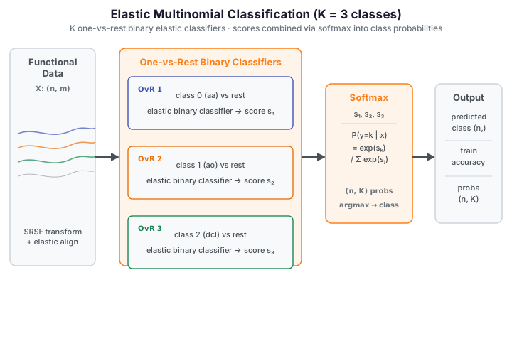
When classes exceed two, elastic_multinomial extends the elastic binary classifier to K classes via a one-vs-rest (OvR) decomposition: it fits K independent binary elastic classifiers (each in the SRSF/elastic domain), then combines their raw scores with a softmax to produce calibrated class probabilities.

Theory

For K classes, let \(s_k(x)\) be the score produced by the \(k\)-th OvR binary elastic classifier applied to curve \(x\). The softmax aggregation yields

\[P(y = k \mid x) = \frac{\exp(s_k(x))}{\sum_{j=1}^{K} \exp(s_j(x))}, \quad k = 1, \dots, K.\]

Each binary classifier uses the same SRSF elastic penalty framework as elastic_logistic, so the model is phase-invariant: time-warping of input curves does not affect the decision boundary.

Parameters

Parameter	Type	Default	Description
data	ndarray (n, m)	—	Functional observations, one per row
labels	ndarray (n,) dtype int64	—	0-indexed contiguous class labels, 0 … K−1
argvals	ndarray (m,)	—	Evaluation grid
ncomp_beta	int	10	B-spline basis functions per OvR classifier
lambda_	float	0.1	Roughness penalty
max_iter	int	100	Maximum IRLS iterations per OvR model
tol	float	1e-4	Convergence tolerance

Returns

Key	Type	Description
n_classes	int	Number of classes K
classes	ndarray (K,)	Unique class indices
train_probabilities	ndarray (n, K)	Softmax class probabilities
predicted_classes	ndarray (n,)	Predicted class label per observation
train_accuracy	float	Resubstitution accuracy

Labels must be 0-indexed contiguous int64 (Pitfall 7)

labels must have dtype np.int64 and contain only the values 0, 1, …, K−1 with no gaps. Passing np.int32, a Python list, or non-contiguous indices (e.g. [0, 2]) raises a ValueError. Remap your class indices to 0 … K−1 before calling:

classes, y = np.unique(raw_labels, return_inverse=True)
y = y.astype(np.int64)

Example: phoneme 3-class classification

The phoneme dataset contains 80 log-periodograms for each of five spoken sounds. We subset to three classes — aa, ao, and dcl — and take 20 observations per class (60 total) so the elastic alignment completes quickly during the docs build. Columns are also downsampled to m ≤ 64.

import numpy as np
from docs_fig import fig, render
from docs_data import load_phoneme
import fdars.classification as clf

freq, X, meta = load_phoneme()
ph = meta["phoneme"].to_numpy()

# 3-class subset: aa, ao, dcl — 20 obs per class for fence speed
classes_3 = ["aa", "ao", "dcl"]
rng = np.random.default_rng(7)
idx = np.concatenate([
    rng.choice(np.where(ph == c)[0], size=20, replace=False) for c in classes_3
])
X3 = X[idx]
y3 = np.array([classes_3.index(ph[i]) for i in idx], dtype=np.int64)
freq3 = freq

# Subsample columns to m <= 64 for fence speed
step = max(1, X3.shape[1] // 64)
X3 = X3[:, ::step]
freq3 = freq3[::step]

res = clf.elastic_multinomial(X3, y3, freq3, ncomp_beta=8, lambda_=0.1)

# Mean spectrum per class
f, ax = fig()
for k, (name, color) in enumerate(zip(classes_3, ["#3f51b5", "#e8710a", "#198754"])):
    ax.plot(freq3, X3[y3 == k].mean(0), color=color, lw=2.2, label=name)
ax.set(title=f"Phoneme 3-class (n_classes={res['n_classes']}, "
             f"accuracy={res['train_accuracy']:.2%})",
       xlabel="frequency index", ylabel="log-periodogram (subsampled)")
ax.legend()
print(render(f))
print(f"n_classes={res['n_classes']}  train_accuracy={res['train_accuracy']:.3f}")
print(f"train_probabilities shape: {np.asarray(res['train_probabilities']).shape}")
print("FDARS_FENCE_OK")

n_classes=3 train_accuracy=1.000 train_probabilities shape: (60, 3) FDARS_FENCE_OK

References

• Delaigle & Hall (2012), JRSS-B.
• Cuevas, Febrero & Fraiman (2007), Computational Statistics.
• Li, Cuesta-Albertos & Liu (2012), DD-classifier, JASA.
• López-Pintado & Romo (2009), functional depth, JASA.