Advanced Elastic Alignment

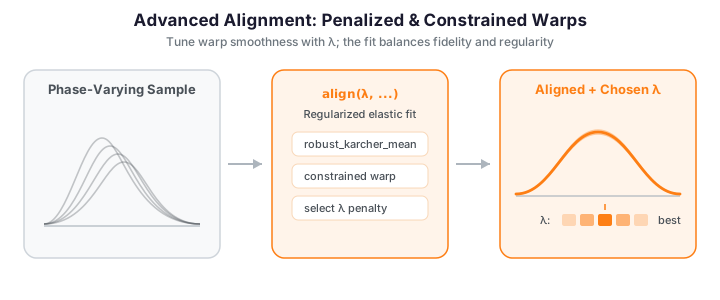
The baseline karcher_mean and elastic_align_pair cover the common case: a smooth warp minimizing the elastic distance with a single smoothness knob, lambda_. Real problems ask for more -- robust estimation under outliers, uncertainty quantification, specialized geometries (closed curves, partial matches), cross-population transfer, generative models, and automatic regularization selection. fdars provides a family of advanced aligners for exactly these cases. Every one operates on the elastic manifold through the SRSF representation \(q(t)=\operatorname{sign}(\dot f(t))\sqrt{|\dot f(t)|}\), which turns the Fisher-Rao metric into the \(L^2\) metric on the Hilbert sphere.

We build a working sample once and reuse it throughout.

The two outliers pull the plain Karcher mean off the true bump; the median and trimmed mean resist them. The rest of this page walks through the advanced tools, grouped as the R reference organizes them.

---

1. Robust central shape: median and trimmed mean

The standard Karcher mean minimizes the sum of squared elastic distances and is therefore sensitive to outliers. Two robust alternatives:

• Karcher median minimizes the sum of unsquared distances via a Weiszfeld iteration on the manifold -- the functional analog of the geometric median.
• Trimmed Karcher mean discards the trim_fraction most distant curves before averaging.

\[ \tilde\mu = \arg\min_{\mu}\sum_{i=1}^n d_e(\mu, f_i) \qquad\text{vs.}\qquad \mu^\* = \arg\min_{\mu}\sum_{i=1}^n d_e(\mu, f_i)^2. \]

from fdars.alignment import karcher_median, robust_karcher_mean

kmed = karcher_median(data, t, max_iter=15)              # robust to outliers
ktrim = robust_karcher_mean(data, t, trim_fraction=0.1)  # drop 10% most distant

mu_median = kmed["mean"]      # elastic median
weights   = kmed["weights"]   # iteratively reweighted per-curve weight
mu_trim   = ktrim["mean"]
kept      = ktrim["weights"]  # 0 for trimmed curves

Both return the same keys as karcher_mean plus weights. See Elastic Alignment for the baseline discussion.

---

2. Elastic depth (phase-aware centrality)

Ordinary functional depth ignores phase: two curves can look equally "central" even though one is a time-warped copy of the other. Elastic depth measures centrality under the elastic metric and decomposes into amplitude and phase parts, so you can spot a curve that is central in shape but outlying in timing.

from fdars.alignment import elastic_depth

ed = elastic_depth(data, t, lambda_=0.0)
amp_depth  = ed["amplitude_depth"]   # (n,)
ph_depth   = ed["phase_depth"]       # (n,)
comb_depth = ed["combined_depth"]    # (n,)
deepest = int(np.argmax(comb_depth))
print(f"Deepest (most central) curve: {deepest}")

Elastic depth is covered in detail, with figures, on the Shape Analysis page.

---

3. Outlier detection (amplitude vs. phase)

elastic_outlier_detection returns, for every curve, its amplitude distance (how unusual its shape is) and its phase distance (how unusual its timing is) relative to a robust reference. Classifying by type means fencing each of these separately -- a plain elastic-distance fence alone will not do it.

The elastic distance is phase-invariant

out["distances"] (and the default out["outlier_indices"]) measure the amplitude distance, which is invariant to time-warping. A curve that is only shifted in time has a near-zero amplitude distance, so it slips through that fence. To catch timing outliers you must look at out["phase_distances"]. Below we inject one amplitude outlier (curve 3, an enlarged bump) and one phase outlier (curve 7, a time-shifted copy) and recover both from the amplitude-vs-phase plane.

import numpy as np
from docs_fig import fig, render
from fdars.alignment import elastic_outlier_detection

rng = np.random.default_rng(7)
n, m = 28, 120
t = np.linspace(0, 1, m)
base = np.exp(-((t - 0.5) ** 2) / (2 * 0.12 ** 2))
data = np.array([rng.normal(1, 0.05) * np.interp(
    t, np.clip(t + rng.normal(0, 0.03), 0, 1), base) for _ in range(n)])
data[3] *= 1.8                                         # amplitude (shape) outlier
data[7] = np.interp(t, np.clip(t - 0.18, 0, 1), base)  # phase (timing) outlier

out = elastic_outlier_detection(data, t, alpha=0.05, use_median=True)
amp = np.asarray(out["amplitude_distances"])   # (n,) shape distance to the reference
pha = np.asarray(out["phase_distances"])       # (n,) timing distance to the reference

def fence(x):                                  # Tukey upper fence (2.0·IQR)
    q1, q3 = np.percentile(x, [25, 75]); return q3 + 2.0 * (q3 - q1)
fa, fp = fence(amp), fence(pha)
amp_out = np.where(amp > fa)[0]                 # unusual shape
pha_out = np.where(pha > fp)[0]                 # unusual timing

f, ax = fig()
ax.scatter(amp, pha, s=26, color="#adb5bd", zorder=2)
ax.axvline(fa, color="#3f51b5", ls="--", lw=1, label="amplitude fence")
ax.axhline(fp, color="#e8710a", ls="--", lw=1, label="phase fence")
for i in amp_out:
    ax.scatter(amp[i], pha[i], s=70, color="#3f51b5", zorder=3)
    ax.annotate(f"{i} · shape", (amp[i], pha[i]), (6, 4),
                textcoords="offset points", fontsize=8, color="#3f51b5")
for i in pha_out:
    ax.scatter(amp[i], pha[i], s=70, color="#e8710a", zorder=3)
    ax.annotate(f"{i} · timing", (amp[i], pha[i]), (6, -11),
                textcoords="offset points", fontsize=8, color="#e8710a")
ax.set(title="Outlier type: amplitude (shape) vs phase (timing)",
       xlabel="amplitude distance", ylabel="phase distance")
ax.legend(fontsize=8)
print(render(f))

print("shape (amplitude) outliers:", list(amp_out),
      " | timing (phase) outliers:", list(pha_out))

shape (amplitude) outliers: [np.int64(3)] | timing (phase) outliers: [np.int64(7)]

Curve 3 lands far to the right (large amplitude distance -> a shape outlier) while curve 7 lands high up (large phase distance -> a timing outlier). Neither fence alone finds both; the amplitude-vs-phase plane separates them cleanly.

Key	Description
outlier_indices	Curves past the amplitude fence (shape outliers only)
distances	Amplitude (elastic) distance of each curve to the reference, shape (n,)
threshold	Tukey fence on distances
amplitude_distances / phase_distances	Per-curve shape / timing distance to the reference, each shape (n,)

---

4. Shape confidence intervals

After computing the Karcher mean, how certain is its shape? shape_confidence_interval gives a bootstrap band: resample the curves, recompute the Karcher mean of each resample, align the bootstrap means to the original mean, and take pointwise percentiles. The alignment step is essential -- without it, phase variability between bootstrap means inflates the band.

import numpy as np
from docs_fig import fig, render
from fdars.alignment import shape_confidence_interval

rng = np.random.default_rng(3)
n, m = 25, 120
t = np.linspace(0, 1, m)
base = np.exp(-((t - 0.5) ** 2) / (2 * 0.12 ** 2))
data = np.array([rng.normal(3, 0.4) * np.interp(
    t, np.clip(t + rng.normal(0, 0.06), 0, 1), base) for _ in range(n)])

ci = shape_confidence_interval(data, t, n_bootstrap=60, confidence_level=0.95,
                               max_iter=10)
mu = np.asarray(ci["mean"])
lo = np.asarray(ci["lower_band"])
hi = np.asarray(ci["upper_band"])

f, ax = fig()
ax.fill_between(t, lo, hi, color="#3f51b5", alpha=0.18, label="95% band")
ax.plot(t, mu, color="#3f51b5", lw=2.2, label="Karcher mean")
ax.set(title="Bootstrap shape confidence interval",
       xlabel="t", ylabel="f(t)")
ax.legend(fontsize=9)
print(render(f))

The shaded band is the pointwise 95% bootstrap envelope around the Karcher mean: where it is narrow the mean shape is well determined, and where it fans out the sample disagrees about amplitude. Because the resampling happens after alignment, the band reflects shape uncertainty rather than leftover phase spread.

Key	Description
mean	The Karcher mean the band is centered on
lower_band / upper_band	Pointwise percentile bands, shape (m,)
bootstrap_means	All bootstrap Karcher means, shape (n_bootstrap, m)

---

5. Bayesian pairwise alignment

Dynamic-programming alignment gives a point estimate of the warp. bayesian_align_pair returns a posterior over warping functions via a Metropolis MCMC sampler on the Hilbert sphere, yielding credible bands and an acceptance rate for diagnostics.

import numpy as np
from docs_fig import fig, render
from fdars.alignment import bayesian_align_pair

t = np.linspace(0, 1, 120)
base = np.exp(-((t - 0.5) ** 2) / (2 * 0.10 ** 2))
f1 = base
f2 = np.interp(t, np.clip(t + 0.08, 0, 1), base)   # phase-shifted target

ba = bayesian_align_pair(f1, f2, t, n_samples=500, burn_in=100, seed=0, step_size=0.85)
f2_aligned = np.asarray(ba["f_aligned_mean"])
gam_lo = np.asarray(ba["credible_lower"])
gam_hi = np.asarray(ba["credible_upper"])
gam_mean = np.asarray(ba["posterior_mean_gamma"])

f, (a1, a2) = fig(ncols=2, figsize=(9.5, 4.0))
a1.plot(t, f1, color="#6c757d", lw=2, label="f1 (reference)")
a1.plot(t, f2, color="#dc3545", lw=1.6, ls="--", label="f2 (original)")
a1.plot(t, f2_aligned, color="#3f51b5", lw=2, label="f2 (aligned)")
a1.set(title=f"Bayesian alignment (accept. {float(ba['acceptance_rate']):.2f})",
       xlabel="t", ylabel="f(t)")
a1.legend(fontsize=8)

a2.fill_between(t, gam_lo, gam_hi, color="#6f42c1", alpha=0.2, label="95% credible")
a2.plot(t, gam_mean, color="#6f42c1", lw=2, label="posterior mean $\\gamma$")
a2.plot([0, 1], [0, 1], color="#6c757d", ls="--", lw=1.2)
a2.set(title="Posterior over the warp", xlabel="t",
       ylabel="$\\gamma(t)$", aspect="equal")
a2.legend(fontsize=8)
print(render(f))

The left panel shows the aligned f2 tracking the reference, while the right panel replaces the single point-estimate warp with a full posterior: the purple band is the 95% credible region around the posterior-mean \(\gamma\). Where the band hugs the diagonal the timing is confidently identity; where it widens the data are ambiguous about how much to warp -- uncertainty a point estimate simply cannot express.

Key	Description
posterior_gammas	MCMC draws of the warp, shape (n_samples, m)
posterior_mean_gamma	Posterior mean warp
credible_lower / credible_upper	Pointwise credible band on the warp
acceptance_rate	MCMC acceptance rate (aim for ~0.2--0.8)
f_aligned_mean	f2 aligned under the posterior-mean warp

Tuning the sampler

If the acceptance rate is too low, reduce step_size; if too high, raise it. Increase n_samples/burn_in for smoother credible bands.

---

6. Multiresolution alignment (long curves)

Dynamic programming is \(O(m^2)\) per pair, slow for long grids. elastic_align_pair_multires aligns a coarsened copy first, then refines on the full grid -- faster and more robust to local minima on long, oscillatory curves. Below, a curve on a 400-point grid is aligned coarse-to-fine and timed against the exact DP solver.

import numpy as np
from time import perf_counter
from docs_fig import fig, render
from fdars.alignment import elastic_align_pair_multires, elastic_align_pair

m = 400                                    # long, oscillatory grid
t = np.linspace(0, 1, m)
base = np.sin(2 * np.pi * 2 * t) + 0.5 * np.sin(2 * np.pi * 5 * t)
f1 = base
f2 = np.interp(t, np.clip(t + 0.09 * np.sin(np.pi * t), 0, 1), base)   # nonlinear phase distortion

t0 = perf_counter()
res = elastic_align_pair_multires(f2, f1, t, coarsen_factor=2,
                                  n_refine_steps=40, step_size=0.1)
t_mr = perf_counter() - t0
f2_aligned = np.asarray(res["f_aligned"]); gamma = np.asarray(res["gamma"])

t0 = perf_counter(); elastic_align_pair(f2, f1, t); t_dp = perf_counter() - t0

f, (a1, a2) = fig(ncols=2, figsize=(9.5, 4.0))
a1.plot(t, f1, color="#6c757d", lw=1.4, label="f1 (reference)")
a1.plot(t, f2, color="#dc3545", lw=1.1, ls="--", alpha=0.8, label="f2 (distorted)")
a1.plot(t, f2_aligned, color="#fd7e14", lw=1.8, label="f2 (aligned)")
a1.set(title=f"Long curves (m={m}) aligned coarse-to-fine", xlabel="t", ylabel="f(t)")
a1.legend(fontsize=8)
a2.plot(t, gamma, color="#fd7e14", lw=2)
a2.plot([0, 1], [0, 1], color="#6c757d", ls="--", lw=1)
a2.set(title=f"Warp γ  ({t_dp / t_mr:.0f}× faster than exact DP)",
       xlabel="t", ylabel="γ(t)", aspect="equal")
print(render(f))

The coarse-to-fine result (orange) recovers the same aligned curve and warp as the exact DP solver but at a fraction of the cost -- the title reports the measured speedup. On a 400-point grid the multiresolution path avoids the full \(O(m^2)\) cost while the S-shaped warp still captures the planted nonlinear phase distortion.

Parameter	Description
coarsen_factor	Grid downsampling factor for the coarse solve (default 4)
n_refine_steps	Gradient refinement steps (default 10)
step_size	Refinement step size (default 0.01)

Returns f_aligned, gamma, distance. The coarse-to-fine result is an approximation of the exact DP solution: it trades a little fidelity for speed, so on short curves prefer the exact elastic_align_pair.

---

7. Closed and periodic curve alignment

A closed curve has no canonical starting point: the same shape can be parameterized from any point on its boundary. elastic_align_pair_closed optimizes over a cyclic start-point rotation \(\theta\) in addition to the warp,

\[ d(f_1, f_2) = \min_{\gamma,\theta}\big\lVert q_1 - (q_2\circ R_\theta\circ\gamma)\sqrt{\dot\gamma}\big\rVert_{L^2}, \]

using a coarse-to-fine search over rotations.

from fdars.alignment import elastic_align_pair_closed

c1 = np.sin(2 * np.pi * t) + 0.3 * np.sin(4 * np.pi * t)
c2 = np.sin(2 * np.pi * (t - 0.1)) + 0.4 * np.sin(4 * np.pi * (t - 0.1))

res = elastic_align_pair_closed(c1, c2, t, lambda_=0.0)
rotation = res["optimal_rotation"]   # best cyclic start-point offset
gamma    = res["gamma"]
distance = res["distance"]

Returns the usual f_aligned, gamma, distance, plus optimal_rotation.

No group periodic=True mode

The R package also exposes a periodic=True circular-rotation mode inside karcher_mean/elastic.align. The Python bindings provide the pairwise closed aligner shown here but no group periodic mode. For a full periodic Karcher mean, pre-rotate each curve (e.g. so its global maximum sits at a fixed grid position) and then call the ordinary karcher_mean.

---

8. Partial matching (subsequence search)

When only a portion of a longer target matches a shorter query, full alignment is wrong. elastic_partial_match finds the best-aligned sub-interval of the target. Here a short query pattern is hidden (time-warped and buried in noise) inside a longer target, and the search recovers exactly where it sits.

import numpy as np
from docs_fig import fig, render
from fdars.alignment import elastic_partial_match

# short query pattern on its own grid
tt = np.linspace(0, 1, 80)
template = np.exp(-((tt - 0.5) ** 2) / (2 * 0.14 ** 2)) * np.sin(2 * np.pi * 2 * tt)

# longer, noisy target; the pattern is embedded (warped) on the sub-interval [0.45, 0.75]
tg = np.linspace(0, 1, 300)
rng = np.random.default_rng(0)
target = 0.15 * rng.standard_normal(300)
seg = (tg >= 0.45) & (tg <= 0.75); s = (tg[seg] - 0.45) / 0.30
target[seg] += 1.2 * np.interp(np.clip(s + 0.05 * np.sin(np.pi * s), 0, 1), tt, template)

pm = elastic_partial_match(template, target, tt, tg, min_span=0.25)
i0, i1 = pm["start_index"], pm["end_index"]

f, ax = fig()
ax.plot(tg, target, color="#adb5bd", lw=1, label="target (long)")
ax.plot(tg[i0:i1 + 1], target[i0:i1 + 1], color="#fd7e14", lw=2.4, label="matched sub-interval")
ax.axvspan(tg[i0], tg[i1], color="#fd7e14", alpha=0.10)
ax.axvspan(0.45, 0.75, color="#198754", alpha=0.06)     # true location (green)
ax.set(title=f"Query found in {pm['domain_fraction']:.0%} of the target  (d={pm['distance']:.2f})",
       xlabel="t", ylabel="f(t)")
ax.legend(fontsize=8)
print(render(f))

print(f"matched target indices {i0}..{i1}  (t = {tg[i0]:.2f}..{tg[i1]:.2f}; planted at 0.45..0.75)")

matched target indices 140..214 (t = 0.47..0.72; planted at 0.45..0.75)

The orange sub-interval that the search selects overlaps the green planted region almost exactly, and the printed indices confirm it recovers the buried pattern despite the noise and time-warping. Crucially the match spans only a fraction of the target (see domain_fraction), which is what distinguishes partial matching from forcing a full-length alignment.

Key	Description
start_index / end_index	Best-matching sub-interval of the target
domain_fraction	Fraction of the target domain that matched
gamma	Warp on the matched segment
distance	Elastic distance of the match

min_span sets the smallest fraction of the target the match may cover, guarding against trivial tiny matches.

---

9. Transfer alignment across populations

When curves come from two populations (healthy vs. diseased, two sites), the population-level shape difference confounds within-subject warping. transfer_alignment maps target curves into the source population's coordinate frame through a bridging warp: align the two Karcher means to get \(\gamma_B\), then compose each target's within-population warp with \(\gamma_B\).

from fdars.alignment import transfer_alignment

source = data[:15]
target = data[15:]

tr = transfer_alignment(source, target, t, max_iter=10)
aligned  = tr["aligned_data"]    # target curves in the source frame
bridging = tr["bridging_gamma"]  # source<-target bridge warp
print(f"Aligned {np.asarray(aligned).shape[0]} target curves to the source frame")

Key	Description
source_mean	Karcher mean of the source population
aligned_data	Target curves placed in the source frame
gammas	Per-curve composed warps \(\gamma_B\circ\gamma_i^T\)
bridging_gamma	The bridge warp aligning target mean to source mean
distances	Elastic distances after transfer

---

10. Geodesic interpolation between curves

A geodesic on the elastic manifold is the shortest path between two shapes -- a natural morph that blends amplitude (in SRSF space) and phase (on the diffeomorphism group). curve_geodesic returns intermediate curves at parameters \(\alpha\in[0,1]\).

import numpy as np
import matplotlib.cm as cm
from docs_fig import fig, render
from fdars.alignment import curve_geodesic

t = np.linspace(0, 1, 140)
f1 = np.exp(-((t - 0.35) ** 2) / 0.01)
f2 = 0.8 * np.exp(-((t - 0.7) ** 2) / 0.006) + 0.4 * np.exp(-((t - 0.3) ** 2) / 0.01)

geo = curve_geodesic(f1, f2, t, n_points=9)
curves = np.asarray(geo["curves"])
alphas = np.asarray(geo["parameter_values"])

f, ax = fig()
for c, a in zip(curves, alphas):
    ax.plot(t, c, color=cm.viridis(a), lw=1.4)
ax.plot(t, f1, color="#3f51b5", lw=2.4, label="$f_1$ ($\\alpha$=0)")
ax.plot(t, f2, color="#dc3545", lw=2.4, label="$f_2$ ($\\alpha$=1)")
ax.set(title="Elastic geodesic: smooth morph $f_1 \\to f_2$",
       xlabel="t", ylabel="f(t)")
ax.legend(fontsize=9)
print(render(f))

The viridis-graded intermediates morph \(f_1\) into \(f_2\) along the shortest elastic path, so the peak migrates smoothly rather than one bump fading while a second grows. That is the elastic geodesic doing its job: it blends amplitude in SRSF space and phase on the warping group simultaneously, unlike a naive pointwise average that would just cross-dissolve the two shapes.

Key	Description
curves	Interpolated curves, shape (n_points, m)
warps	The intermediate warps
distances	Cumulative elastic distance along the path
parameter_values	The \(\alpha\in[0,1]\) for each curve

---

11. Gaussian generative model

After separating amplitude and phase, you can generate new curves by sampling from the estimated score distributions -- useful for augmentation and simulation. gauss_model fits Gaussians to the vertical (amplitude) and horizontal (phase) FPC scores and draws new samples; joint_gauss_model fits a joint Gaussian that preserves amplitude-phase correlation.

import numpy as np
from docs_fig import fig, render
from fdars.alignment import gauss_model

rng = np.random.default_rng(1)
n, m = 30, 120
t = np.linspace(0, 1, m)
base = np.exp(-((t - 0.5) ** 2) / (2 * 0.12 ** 2))
data = np.array([rng.normal(3, 0.4) * np.interp(
    t, np.clip(t + rng.normal(0, 0.06), 0, 1), base) for _ in range(n)])

gm = gauss_model(data, t, ncomp=3, n_samples=20, max_iter=15, seed=0)
synth = np.asarray(gm["samples"])

f, ax = fig()
ax.plot(t, data.T, color="#3f51b5", lw=0.8, alpha=0.35)
ax.plot(t, synth.T, color="#e8710a", lw=0.8, alpha=0.5)
ax.plot([], [], color="#3f51b5", lw=2, label="original")
ax.plot([], [], color="#e8710a", lw=2, label="generated")
ax.set(title="Gaussian generative model: original vs. synthetic",
       xlabel="t", ylabel="f(t)")
ax.legend(fontsize=9)
print(render(f))

The orange synthetic curves occupy the same amplitude-and-timing envelope as the blue originals -- the generative model has learned the joint distribution of shape and phase rather than memorizing individual curves. This is the payoff of the amplitude/phase separation: sampling the two score distributions produces plausible new curves for augmentation or simulation.

Key	Description
samples	Synthetic curves, shape (n_samples, m)
warps	Warps applied to the synthetic amplitudes
scores	Sampled FPC scores

---

12. Peak persistence for automatic \(\lambda\)

Choosing the regularization \(\lambda\) is usually ad hoc. Peak persistence offers a topological criterion: sweep \(\lambda\), track when peaks in the Karcher mean are born and die, and pick the \(\lambda\) where persistent (genuine) peaks survive but transient (noise) peaks have merged away.

from fdars.alignment import peak_persistence

lambdas = np.linspace(0.0, 3.0, 15)   # must be an ndarray
pers = peak_persistence(data, t, lambdas=lambdas, max_iter=8)
print(f"Optimal lambda: {float(pers['optimal_lambda']):.3f}")
print(f"Peak counts:    {list(np.asarray(pers['peak_counts'], dtype=int))}")

Key	Description
lambdas	The swept grid
peak_counts	Number of Karcher-mean peaks at each \(\lambda\)
optimal_lambda / optimal_index	Selected regularization and its grid index

Cross-validation (next section) optimizes a reconstruction score; peak persistence optimizes topological stability. They answer slightly different questions -- use CV when you have a clear predictive target, persistence when you care about recovering the right number of features.

---

13. Choosing \(\lambda\) by cross-validation

lambda_cv scores a grid of regularization values by \(K\)-fold cross-validation over the whole dataset and reports the best one.

import numpy as np
from docs_fig import fig, render
from fdars.alignment import lambda_cv

rng = np.random.default_rng(7)
n, m = 20, 100
t = np.linspace(0, 1, m)
base = np.exp(-((t - 0.35) ** 2) / 0.01) + 0.6 * np.exp(-((t - 0.7) ** 2) / 0.008)
data = np.zeros((n, m))
for i in range(n):
    warp = t ** rng.uniform(0.7, 1.5)
    warp = (warp - warp.min()) / np.ptp(warp)
    data[i] = np.interp(t, warp, base)

lambdas = np.array([0.0, 0.001, 0.01, 0.05, 0.1, 0.5])   # must be an ndarray
cv = lambda_cv(data, t, lambdas=lambdas, n_folds=3, max_iter=10, tol=1e-3)

best = float(cv["best_lambda"])
f, ax = fig()
ax.plot(cv["lambdas"], cv["cv_scores"], "o-", color="#3f51b5", lw=1.8)
ax.axvline(best, color="#e8710a", ls="--", lw=1.5, label=f"best $\\lambda$={best:g}")
ax.set(title="Cross-validated warp regularization", xlabel="$\\lambda$",
       ylabel="CV score (lower is better)")
ax.legend(fontsize=9)
print(render(f))

The CV curve dips to a minimum at the selected \(\lambda\) (orange line): too little regularization overfits the warps to noise, too much stiffens them toward the identity and leaves curves misaligned. The valley is the sweet spot that generalizes best across the held-out folds.

Key	Description
best_lambda	Regularization minimizing the CV score
cv_scores	Mean CV score for each candidate
lambdas	The candidate grid that was scored

Array arguments must be ndarray

lambda_cv, peak_persistence, and elastic_align_pair_constrained reject plain Python lists for their array arguments (lambdas, landmark_targets, landmark_sources) with a TypeError. Wrap them with np.array(...).

---

Pairwise variants and their penalties

Beyond the specialized aligners above, fdars exposes the pairwise objective's regularization directly. Every pairwise aligner minimizes an elastic objective in SRSF space,

\[ \gamma^\* = \arg\min_{\gamma}\;\big\lVert q_1 - (q_2\circ\gamma)\sqrt{\dot\gamma}\big\rVert_{L^2}^2 \;+\; \lambda\,\mathcal{P}(\gamma), \]

and the variants differ in the roughness penalty \(\mathcal{P}\) and the constraints on \(\gamma\). The figure shows how \(\lambda\) moves the estimated warp between an unconstrained fit and the identity.

import numpy as np
from docs_fig import fig, render
from fdars.alignment import elastic_align_pair_penalized

t = np.linspace(0, 1, 120)
base = np.exp(-((t - 0.4) ** 2) / 0.01) + 0.7 * np.exp(-((t - 0.75) ** 2) / 0.006)
warp = t ** 1.5
warp = (warp - warp.min()) / np.ptp(warp)
target = base
source = np.interp(t, warp, base)

f, ax = fig()
colors = {"0.0": "#dc3545", "0.05": "#e8710a", "0.5": "#198754", "5.0": "#6f42c1"}
labels = {"0.0": "under (λ=0)", "0.05": "well (λ=0.05)",
          "0.5": "strong (λ=0.5)", "5.0": "over (λ=5)"}
for lam_s, c in colors.items():
    res = elastic_align_pair_penalized(source, target, t, lambda_=float(lam_s))
    ax.plot(t, np.asarray(res["gamma"]), color=c, lw=1.8, label=labels[lam_s])
ax.plot([0, 1], [0, 1], color="#6c757d", lw=1.3, ls="--", label="identity")
ax.set(title="Warp $\\gamma$ vs. penalty $\\lambda$", xlabel="t",
       ylabel="$\\gamma(t)$", aspect="equal")
ax.legend(fontsize=8)
print(render(f))

As \(\lambda\) grows the warp is pulled toward the diagonal: too small and it over-fits noise, too large and it collapses to the identity (no alignment).

Penalized

Choose the penalty functional. first_order penalizes the warp's departure from the identity in slope; second_order penalizes curvature (favoring smoother, gently bending warps); second_order_weight blends the two.

from fdars.alignment import elastic_align_pair_penalized

res = elastic_align_pair_penalized(
    f2, f1, t, lambda_=0.1,
    penalty_type="second_order",   # or "first_order" (default)
    second_order_weight=0.1,
)
gamma = res["gamma"]

Landmark-constrained

When you already know that specific features correspond (a shared peak), pin them. The warp is forced through the given (source, target) landmark pairs and optimized elastically between them.

from fdars.alignment import elastic_align_pair_constrained

# landmark arrays MUST be ndarrays (a Python list raises TypeError)
src = np.array([0.55])   # landmark location in f2
tgt = np.array([0.50])   # where it should map to in f1

res = elastic_align_pair_constrained(f1, f2, t, tgt, src, lambda_=0.0)
gamma = res["gamma"]     # satisfies gamma(tgt) = src at the knots

Parameter	Description
landmark_targets	Target landmark locations (must be ndarray)
landmark_sources	Source landmark locations (must be ndarray)
lambda_	Warp regularization

For pure landmark warping

elastic_align_pair_constrained pins landmarks within an elastic fit. For a pure monotone landmark warp with no elastic optimization, see Landmark Registration.

All pairwise variants return at least f_aligned, gamma, and distance; closed adds optimal_rotation.

---

Binding gaps vs. the R reference

Two R advanced features have no Python binding and are omitted here rather than faked:

• Multivariate (vector-valued) alignment -- karcher.mean.nd / pca.nd. Even in R these are noted as "wrappers pending"; the fdars Python surface is scalar-curve only.
• Group periodic mode -- periodic=True inside karcher_mean. The pairwise closed aligner is available; the group periodic Karcher mean is not (workaround noted there).

Horizontal FPNS (horiz_fpns) is bound and is covered on the Shape Analysis page alongside horizontal FPCA.

---

See Elastic Alignment for the baseline aligner and the SRSF/Karcher-mean machinery, TSRVF for linearized statistics, Shape Analysis for elastic FPCA and depth, and Comparing Alignment Methods for how these fits stack up against landmark registration.

References

• Fletcher, P.T., Venkatasubramanian, S., Joshi, S. (2009). The geometric median on Riemannian manifolds. NeuroImage 45(1):S143-S152.
• Cheng, W., Dryden, I.L., Huang, X. (2016). Bayesian registration of functions and curves. Bayesian Analysis 11(2):447-481.
• Tucker, J.D., Wu, W., Srivastava, A. (2013). Generative models for functional data using phase and amplitude separation. Computational Statistics & Data Analysis 61:50-66.
• Srivastava, A., Klassen, E. (2016). Functional and Shape Data Analysis. Springer.