PACE — FPCA for Sparse, Irregular Data

PACE (Principal Analysis by Conditional Expectation) extends functional PCA to the realistic setting where each curve is observed at its own sparse, irregular grid — not on a shared dense grid. Clinical longitudinal studies, sensor networks with missed readings, and ecological monitoring data all produce this kind of input. Standard FPCA requires a common grid and breaks when curves have different numbers of observations at different locations. PACE handles it correctly.

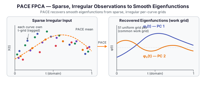
The key idea: PACE first estimates the population mean and covariance surface nonparametrically from all available observation pairs, then recovers individual FPC scores via conditional expectation given the sparse observations. The result is a set of smooth eigenfunctions on a common work grid, plus scores and fitted curves for every observation — even those with only a handful of measurement points.

Theory

Every square-integrable random function \(X_i(t)\) admits the Karhunen-Loève expansion

\[ X_i(t) = \mu(t) + \sum_{k=1}^{\infty} \xi_{ik}\,\phi_k(t) \]

where \(\mu(t)\) is the population mean, \(\phi_k(t)\) the \(k\)-th eigenfunction of the covariance operator, and \(\xi_{ik}\) the corresponding score. With dense, regular observations we estimate the covariance directly from the data matrix. With sparse, irregular observations we cannot: different curves are observed at different time points, so the sample covariance matrix is largely missing.

PACE estimates the covariance surface \(C(s,t)\) by local linear smoothing of all cross-product pairs \((X_i(s_j),\, X_i(t_k))\) at distinct time pairs \((s_j, t_k)\) within each curve, pooled across curves. The diagonal (measurement error) is handled separately. Eigen-decomposition of the estimated surface yields \(\hat\phi_k\) and \(\hat\lambda_k\) on the common work grid.

Scores are then recovered by conditional expectation:

\[ \hat\xi_{ik} = \hat\lambda_k\,\hat\phi_k^\top \boldsymbol{\Sigma}_i^{-1}\bigl(\mathbf{y}_i - \hat\boldsymbol{\mu}_i\bigr) \]

where \(\mathbf{y}_i\) is the vector of observed values for curve \(i\), \(\hat\boldsymbol{\mu}_i\) is the mean evaluated at those time points, and \(\boldsymbol{\Sigma}_i = \hat\lambda_k\hat\phi_k\hat\phi_k^\top + \hat\sigma^2 I\) is the marginal covariance at the observed locations.

irreg_fdata_from_lists — building the sparse input handle

Parameter	Type	Description
argvals_list	list[ndarray (n_i,)]	List of 1-D arrays — evaluation grid for curve \(i\) (ragged; lengths may differ)
values_list	list[ndarray (n_i,)]	List of 1-D arrays — observed values for curve \(i\) (must match argvals_list[i] in length)

Returns an opaque PyIrregFdata handle for use with pace_fpca.

2-D numpy arrays are rejected

irreg_fdata_from_lists requires two Python lists of 1-D arrays — one list per curve for the grid and one for the values. Passing a dense 2-D numpy array (n, m) raises a ValueError. Build the lists explicitly before calling the function.

pace_fpca — fitting PACE-FPCA

Parameter	Type	Default	Description
data	PyIrregFdata	—	Handle from irreg_fdata_from_lists
ncomp	int	3	Number of principal components to request
bandwidth	float	0.1	Kernel bandwidth for covariance surface smoothing; increase for sparser data (≥ 0.15 recommended for data on [0, 1] with few points per curve)
sigma2	float	0.01	Measurement error variance; increase if observations are noisy
work_grid	list[float] \| None	None	Evaluation grid for mean and eigenfunctions; None → 51 uniformly spaced points on [0, 1]
alpha	float	0.05	Significance level for pointwise confidence bands

Returns

Key	Shape	Description
mean	(m,)	Estimated mean function on the work grid
eigenvalues	(ncomp,)	Eigenvalues \(\hat\lambda_1 \ge \hat\lambda_2 \ge \cdots\)
eigenfunctions	(m, ncomp)	Estimated eigenfunctions; column \(k\) is the \(k\)-th eigenfunction \(\hat\phi_{k+1}(t)\)
scores	(n, ncomp)	Conditional-expectation FPC scores \(\hat\xi_{ik}\)
fitted	(n, m)	Fitted curves \(\hat\mu(t) + \sum_k \hat\xi_{ik}\hat\phi_k(t)\) on the work grid
fitted_lower	(n, m)	Lower pointwise confidence band for each fitted curve
fitted_upper	(n, m)	Upper pointwise confidence band for each fitted curve
argvals	(m,)	Work grid used for all function evaluations
sigma2	float	Estimated measurement error variance (may differ from the input if re-estimated)
ncomp	int	Actual number of components retained (may be less than requested if the covariance estimate has fewer positive eigenvalues)

Actual component count

The ncomp value in the returned dict is the actual count of components retained and may be less than the requested ncomp parameter. Always read res["ncomp"] to determine the true length of the eigenvalues array and the number of columns in eigenfunctions and scores.

Example — synthetic sparse irregular data

import numpy as np
from docs_fig import fig, render
import fdars.pace_fpca as pf

rng = np.random.default_rng(42)
n = 15  # sparse curves; each has only 5-8 observations

# Build ragged per-curve grids: different number of points, different positions per curve
argvals_list = [np.sort(rng.uniform(0, 1, rng.integers(5, 9))) for _ in range(n)]
values_list  = [np.sin(2 * np.pi * av) + rng.normal(0, 0.15, len(av))
                for av in argvals_list]

# IMPORTANT: pass Python lists of 1-D arrays — NOT a 2-D numpy array
handle = pf.irreg_fdata_from_lists(argvals_list, values_list)
res = pf.pace_fpca(handle, ncomp=2, bandwidth=0.2, sigma2=0.05)

ef = np.asarray(res["eigenfunctions"])   # shape (m, ncomp) — column k is PC k
argvals_out = np.asarray(res["argvals"]) # common work grid

f, (a0, a1) = fig(1, 2, figsize=(11.0, 3.8))

# Left: scatter sparse observations per curve + PACE mean
for av, vl in zip(argvals_list, values_list):
    a0.scatter(av, vl, s=18, color="#3f51b5", alpha=0.45)
a0.plot(argvals_out, np.asarray(res["mean"]), color="#e8710a", lw=2.4, label="PACE mean")
a0.set(title=f"Sparse irregular observations (n={n}, ragged grids)", xlabel="t")
a0.legend(fontsize=9)

# Right: recovered smooth eigenfunctions on common work grid
a1.plot(argvals_out, ef[:, 0], color="#3f51b5", lw=2.4, label="PC 1")
a1.plot(argvals_out, ef[:, 1], color="#e8710a", lw=2.4, label="PC 2")
a1.axhline(0, color="#ced4da", lw=0.8, ls="--")
a1.set(title="PACE eigenfunctions recovered on work grid", xlabel="t")
a1.legend(fontsize=9)

print(render(f))
print(f"actual ncomp={res['ncomp']}  scores shape={np.asarray(res['scores']).shape}")
print("FDARS_FENCE_OK")

actual ncomp=2 scores shape=(15, 2) FDARS_FENCE_OK

PACE vs standard FPCA

Standard FPCA (fdars.regression.fpca) assumes every curve is observed at the same dense common grid — it operates on a full \(n \times m\) matrix. When curves are sparse or ragged, the matrix cannot be formed, and reg.fpca fails or requires imputation that distorts the covariance structure.

PACE recovers the population mean and covariance surface directly from pooled sparse observation pairs, then extracts scores by conditional expectation — it never requires a complete data matrix. The table below summarises the trade-offs:

Aspect	reg.fpca (standard)	pf.pace_fpca (PACE)
Input	Dense (n, m) matrix (common grid)	PyIrregFdata handle (ragged grids)
Minimum obs. per curve	All \(m\) points	As few as 2–3 per curve
Covariance estimation	Direct from data matrix	Local linear smoothing of pooled pairs
Score recovery	Truncated KL projection	Conditional expectation (BLUP)
Key parameter	n_comp	ncomp, bandwidth, sigma2

When PACE helps vs basis smoothing

PACE is the right choice when curves are observed at sparse, irregular, ragged time points and the measurement error is non-negligible. It can fail if:

• Too few points per curve (fewer than 2–3): the conditional-expectation formula becomes ill-conditioned and scores are unreliable.
• Bandwidth too small for the sparsity level: the covariance surface smoother cannot see enough pooled pairs, producing a noisy covariance estimate. A bandwidth around 0.15–0.3 of the domain width is a safe starting point for data on \([0, 1]\) with 5–10 points per curve (see bandwidth guidance in the pace_fpca parameters table above).

When curves are dense but observed on non-uniform individual grids, consider basis smoothing (e.g., fdars.smoothing) to interpolate to a common grid first, then run reg.fpca. The PACE kernel smoother adds bandwidth-tuning overhead that is unnecessary if the data is merely irregular rather than sparse.

Example — comparing PACE and standard FPCA on the same data

The fence below builds one small synthetic dense dataset, runs reg.fpca on the full matrix, then subsamples each curve to a ragged sparse set and runs pf.pace_fpca. It compares the leading eigenfunction (correlation, up to sign) and leading eigenvalue from each method to show that PACE recovers a consistent estimate from sparse observations.

import numpy as np
from docs_fig import fig, render, fast
import fdars.regression as reg
import fdars.pace_fpca as pf

rng = np.random.default_rng(7)
n, m = 15, 40
t = np.linspace(0, 1, m)

# Dense synthetic dataset (two-component KL model)
phi1 = np.sqrt(2) * np.sin(2 * np.pi * t)
phi2 = np.sqrt(2) * np.cos(2 * np.pi * t)
scores_true = rng.normal(0, 1, (n, 2)) * np.array([[1.5, 0.8]])
X_dense = scores_true[:, 0:1] * phi1 + scores_true[:, 1:2] * phi2
X_dense += rng.normal(0, 0.1, X_dense.shape)

# --- Standard FPCA on the full dense matrix ---
res_fpca = reg.fpca(X_dense, t, n_comp=2)
ef_dense = np.asarray(res_fpca["rotation"])    # (m, 2) — column k is PC k
sv_dense = np.asarray(res_fpca["singular_values"])  # (2,) singular values

# Eigenvalues from standard FPCA (singular_values are sqrt(n*lambda_k))
eig_dense = sv_dense ** 2 / n

# --- PACE-FPCA on the sparse subsampled version ---
# Subsample each curve to 5-8 irregular points
argvals_list = [np.sort(rng.choice(t, size=rng.integers(5, 9), replace=False))
                for _ in range(n)]
values_list  = [np.interp(av, t, X_dense[i]) + rng.normal(0, 0.1, len(av))
                for i, av in enumerate(argvals_list)]

handle = pf.irreg_fdata_from_lists(argvals_list, values_list)
bw = fast(0.25, 0.25)
res_pace = pf.pace_fpca(handle, ncomp=2, bandwidth=bw, sigma2=0.05,
                        work_grid=list(t))
ef_pace = np.asarray(res_pace["eigenfunctions"])  # (m, ncomp)
eig_pace = np.asarray(res_pace["eigenvalues"])     # (ncomp,)

# Leading eigenfunctions: correlate (up to sign) — both should be close to phi1
ef1_dense = ef_dense[:, 0]
ef1_pace  = ef_pace[:, 0]
sign = np.sign(np.dot(ef1_dense, ef1_pace))
corr_pc1 = np.dot(ef1_dense, sign * ef1_pace) / (
    np.linalg.norm(ef1_dense) * np.linalg.norm(ef1_pace)
)

f, (a0, a1) = fig(1, 2, figsize=(12.0, 3.8))

a0.plot(t, ef1_dense, color="#3f51b5", lw=2.2, label="Standard FPCA (dense)")
a0.plot(t, sign * ef1_pace, color="#e8710a", lw=2.2, ls="--", label="PACE (sparse)")
a0.set(title=f"PC 1 comparison  (corr={corr_pc1:.3f})", xlabel="t",
       ylabel="eigenfunction")
a0.legend(fontsize=9)

a1.bar(["PC 1", "PC 2"], eig_dense[:2], color="#3f51b5", alpha=0.7,
       label="Standard FPCA")
a1.bar(["PC 1", "PC 2"], eig_pace[:2], color="#e8710a", alpha=0.55,
       label="PACE", width=0.4, align="edge")
a1.set(title="Leading eigenvalues", ylabel="eigenvalue")
a1.legend(fontsize=9)

print(render(f))
print(f"Standard FPCA  eig1={eig_dense[0]:.3f}  eig2={eig_dense[1]:.3f}")
print(f"PACE           eig1={eig_pace[0]:.3f}  eig2={eig_pace[1]:.3f}")
print(f"PC 1 alignment: corr(dense, pace)={corr_pc1:.3f} (close to ±1 when PACE recovers well)")
print("FDARS_FENCE_OK")

Standard FPCA eig1=1.808 eig2=0.254 PACE eig1=0.865 eig2=0.151 PC 1 alignment: corr(dense, pace)=0.829 (close to ±1 when PACE recovers well) FDARS_FENCE_OK

References

1. Yao, F., Müller, H.-G. & Wang, J.-L. (2005). Functional data analysis for sparse longitudinal data. Journal of the American Statistical Association, 100(470), 577–590.
2. Hall, P., Müller, H.-G. & Wang, J.-L. (2006). Properties of principal component methods for functional and longitudinal data analysis. The Annals of Statistics, 34(3), 1493–1517.