Andrews Transformation: From Tables to Curves

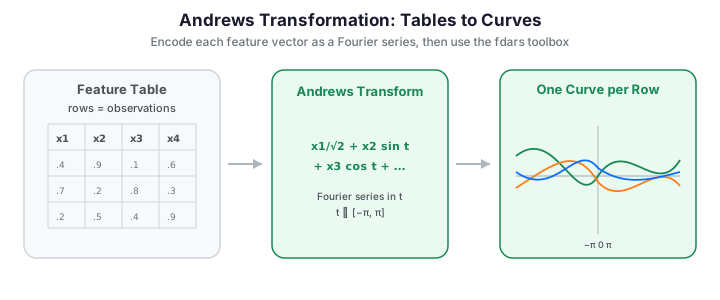
An Andrews transformation maps each row of a multivariate data table -- a plain feature vector \(x = (x_1, x_2, \ldots, x_p)\) -- to a smooth periodic curve. Introduced by David Andrews in 1972 as a way to visualize high-dimensional data, it turns out to be a bridge into functional data analysis: once every observation is a curve, the whole fdars toolbox (depth, distances, clustering, outlier detection) applies to ordinary tabular data. This page shows the transform explicitly in numpy, then analyzes the resulting curves with real fdars functions.

No andrews binding in the Python fdars

The R package ships a dedicated andrews_transform(), but the Python fdars has no Andrews-curve function. The transform is a handful of lines of numpy, shown in full below. fdars enters only after the transform, once the curves are wrapped in Fdata.

The transform

Andrews encodes the feature vector as the coefficients of a truncated Fourier series in a dummy variable \(t \in [-\pi, \pi]\):

\[ f_x(t) = \frac{x_1}{\sqrt{2}} + x_2 \sin t + x_3 \cos t + x_4 \sin 2t + x_5 \cos 2t + \cdots \]

Each observation becomes one curve \(f_x(t)\). The construction has two properties that make it useful rather than arbitrary:

• Distance preservation. By Parseval's theorem the \(L^2\) distance between two Andrews curves is proportional to the Euclidean distance between their feature vectors:

  \[ \int_{-\pi}^{\pi} \bigl(f_x(t) - f_y(t)\bigr)^2\,dt = \pi\,\lVert x - y\rVert_2^2 \quad\Longrightarrow\quad \lVert f_x - f_y\rVert_{L^2} = \sqrt{\pi}\,\lVert x - y\rVert_2 . \]

  Curves that look similar correspond to observations that are similar, and every distance-based method (depth, clustering) is interpretable back in the original feature space up to the constant \(\sqrt{\pi}\). - Mean preservation. The Andrews curve of the sample mean equals the mean of the Andrews curves, so a "central" curve is a central observation.

Here is the entire transform in numpy -- there is no hidden machinery:

import numpy as np
from docs_fig import fig, render

def andrews_curves(features, t):
    """Map rows of a (n, p) table to Andrews curves evaluated at t.

    f_x(t) = x1/sqrt(2) + x2 sin t + x3 cos t + x4 sin 2t + x5 cos 2t + ...
    """
    features = np.asarray(features, float)
    n, p = features.shape
    out = np.full((n, t.size), features[:, [0]] / np.sqrt(2.0))
    for j in range(1, p):
        harmonic = (j + 1) // 2               # 1,1,2,2,3,3,...
        term = np.sin if j % 2 == 1 else np.cos
        out = out + features[:, [j]] * term(harmonic * t)
    return out

# A small synthetic table: 3 groups in a 4-dimensional feature space.
rng = np.random.default_rng(7)
group_means = np.array([[ 2.0,  0.0,  1.0,  0.0],
                        [ 0.0,  2.0,  0.0,  1.0],
                        [-2.0, -1.0,  1.0, -1.0]])
features = np.vstack([mu + 0.4 * rng.standard_normal((10, 4))
                      for mu in group_means])
labels = np.repeat([0, 1, 2], 10)

t = np.linspace(-np.pi, np.pi, 120)
curves = andrews_curves(features, t)          # (30, 120)

colors = ["#3f51b5", "#e8710a", "#198754"]
f, ax = fig()
for i in range(curves.shape[0]):
    ax.plot(t, curves[i], color=colors[labels[i]], lw=1, alpha=0.6)
ax.set(title="Andrews curves of a 3-group feature table",
       xlabel="t", ylabel=r"$f_x(t)$")
print(render(f))

The three colored bundles are already visible: rows from the same group in feature space trace out similar curves, because the transform preserves distances.

Wrapping curves in Fdata

From here on the data is functional. Bundle the curves into an fdars.Fdata object and every method of the class becomes available.

import numpy as np
from fdars import Fdata

fd = Fdata(curves, argvals=t)
print(fd.n_obs(), "curves on", fd.n_points(), "points")

Step	Object	Notes
Feature table	np.ndarray (n, p)	Any multivariate data set
andrews_curves(...)	np.ndarray (n, m)	Pure numpy, shown above
Fdata(curves, argvals=t)	fdars.Fdata	Enables depth, distance, clustering

Depth: finding the central observation and outliers

Because Andrews curves preserve distances, functional depth of a curve is a sensible centrality measure for the underlying feature vector. The deepest curve is the "most typical" row; shallow curves flag multivariate outliers. We use modified_band_1d from fdars.depth.

import numpy as np
from docs_fig import fig, render
from fdars.depth import modified_band_1d

def andrews_curves(features, t):
    features = np.asarray(features, float)
    n, p = features.shape
    out = np.full((n, t.size), features[:, [0]] / np.sqrt(2.0))
    for j in range(1, p):
        harmonic = (j + 1) // 2
        term = np.sin if j % 2 == 1 else np.cos
        out = out + features[:, [j]] * term(harmonic * t)
    return out

rng = np.random.default_rng(7)
group_means = np.array([[ 2.0,  0.0,  1.0,  0.0],
                        [ 0.0,  2.0,  0.0,  1.0],
                        [-2.0, -1.0,  1.0, -1.0]])
features = np.vstack([mu + 0.4 * rng.standard_normal((10, 4))
                      for mu in group_means])
# Inject one clear multivariate outlier
features = np.vstack([features, np.array([6.0, -5.0, 4.0, 5.0])])

t = np.linspace(-np.pi, np.pi, 120)
curves = andrews_curves(features, t)
depth = np.asarray(modified_band_1d(curves, curves))
order = np.argsort(depth)
rng_d = np.ptp(depth) + 1e-9

f, ax = fig()
for i in order:                                    # faint = shallow (outlying)
    ax.plot(t, curves[i], color="#3f51b5", lw=1.1,
            alpha=0.15 + 0.8 * (depth[i] - depth.min()) / rng_d)
ax.plot(t, curves[order[-1]], color="#198754", lw=2.4, label="deepest (typical)")
ax.plot(t, curves[order[0]], color="#dc3545", lw=2.4, label="shallowest (outlier)")
ax.set(title="Depth of Andrews curves flags a multivariate outlier",
       xlabel="t", ylabel=r"$f_x(t)$")
ax.legend()
print(render(f))

The injected outlier receives the lowest depth and stands out as the red curve -- multivariate outlier detection carried out entirely through the functional representation.

Distances and clustering

The distance-preservation property means we can cluster the curves and recover the groups in the feature table. Using kmeans_fd from fdars.clustering on the Andrews curves reproduces the three groups.

import numpy as np
from docs_fig import fig, render
from fdars.clustering import kmeans_fd

def andrews_curves(features, t):
    features = np.asarray(features, float)
    n, p = features.shape
    out = np.full((n, t.size), features[:, [0]] / np.sqrt(2.0))
    for j in range(1, p):
        harmonic = (j + 1) // 2
        term = np.sin if j % 2 == 1 else np.cos
        out = out + features[:, [j]] * term(harmonic * t)
    return out

rng = np.random.default_rng(7)
group_means = np.array([[ 2.0,  0.0,  1.0,  0.0],
                        [ 0.0,  2.0,  0.0,  1.0],
                        [-2.0, -1.0,  1.0, -1.0]])
features = np.vstack([mu + 0.4 * rng.standard_normal((10, 4))
                      for mu in group_means])
t = np.linspace(-np.pi, np.pi, 120)
curves = andrews_curves(features, t)

km = kmeans_fd(curves, t, k=3)
cluster = np.asarray(km["cluster"])
centers = np.asarray(km["centers"])

palette = ["#3f51b5", "#e8710a", "#198754"]
f, ax = fig()
for i in range(curves.shape[0]):
    ax.plot(t, curves[i], color=palette[cluster[i]], lw=0.9, alpha=0.4)
for c in range(3):
    ax.plot(t, centers[c], color=palette[c], lw=2.6)
ax.set(title="kmeans_fd on Andrews curves recovers the 3 feature-space groups",
       xlabel="t", ylabel=r"$f_x(t)$")
print(render(f))

The bold curves are the cluster centroids in curve space; each corresponds to one group centroid in the original 4-dimensional table. Because the transform is linear, the centroid curve is exactly the Andrews curve of the feature-space centroid.

Ordering matters for plots, not for analysis

Andrews curves are not invariant to the order of the features: \(x_1\) (the constant term) and the low harmonics (\(x_2, x_3\)) dominate the curve's shape, while high-index features contribute fast wiggles that are easy to overlook. Put the most informative variables first (rank them by, e.g., variance or an ANOVA \(F\)-statistic), and standardize columns beforehand so no single feature swamps the rest. Crucially, because the transform preserves distances exactly, reordering changes only the picture -- any distance-based result (clustering assignments, depth ranks) is identical whatever the column order.

Verifying distance preservation on a real table

The \(\sqrt{\pi}\) relationship is not a heuristic -- it holds to machine precision. Here it is checked on the Wine dataset (178 wines, 13 standardized chemical features): every pairwise Andrews \(L^2\) distance, computed with lp_self_1d, equals exactly \(\sqrt{\pi}\) times the Euclidean distance between the underlying feature vectors.

import numpy as np
from docs_fig import fig, render
from docs_data import load_wine
from fdars.metric import lp_self_1d

names, X_raw, meta = load_wine()
X = (X_raw - X_raw.mean(0)) / X_raw.std(0)      # standardize columns

def andrews_curves(features, t):
    features = np.asarray(features, float)
    n, p = features.shape
    out = np.full((n, t.size), features[:, [0]] / np.sqrt(2.0))
    for j in range(1, p):
        harmonic = (j + 1) // 2
        term = np.sin if j % 2 == 1 else np.cos
        out = out + features[:, [j]] * term(harmonic * t)
    return out

t = np.linspace(-np.pi, np.pi, 200)
curves = andrews_curves(X, t)

D_andrews = np.asarray(lp_self_1d(curves, t, p=2.0))     # functional L2 distances
diff = X[:, None, :] - X[None, :, :]
D_euclid = np.sqrt((diff ** 2).sum(-1))                 # Euclidean distances

iu = np.triu_indices(X.shape[0], k=1)
da, de = D_andrews[iu], D_euclid[iu]
nz = de > 1e-10
ratio = da[nz] / de[nz]

f, ax = fig(figsize=(5.5, 5.5))
ax.scatter(de[nz], da[nz], s=4, alpha=0.12, color="#3f51b5")
xs = np.array([0.0, de[nz].max()])
ax.plot(xs, np.sqrt(np.pi) * xs, color="#dc3545", lw=1.8,
        label=r"slope $\sqrt{\pi}\approx$" + f"{np.sqrt(np.pi):.4f}")
ax.set(title=f"Andrews $L^2$ vs Euclidean (mean ratio {ratio.mean():.4f})",
       xlabel="Euclidean distance (standardized features)",
       ylabel="Andrews $L^2$ distance")
ax.legend()
print(render(f))

Every point falls on the red line: the transform is an isometry up to \(\sqrt{\pi}\).

FPCA on Andrews curves recovers the classes

Because the transform is an isometry, running functional PCA on the Wine Andrews curves is equivalent to PCA on the standardized table -- but it comes for free from the same Fdata pipeline. The score plot below colours each wine by its (unused) cultivar label to check that the leading functional principal components separate the three known groups.

import numpy as np
from docs_fig import fig, render
from docs_data import load_wine
from fdars.regression import fpca

names, X_raw, meta = load_wine()
X = (X_raw - X_raw.mean(0)) / X_raw.std(0)      # standardize columns

def andrews_curves(features, t):
    features = np.asarray(features, float)
    n, p = features.shape
    out = np.full((n, t.size), features[:, [0]] / np.sqrt(2.0))
    for j in range(1, p):
        harmonic = (j + 1) // 2
        term = np.sin if j % 2 == 1 else np.cos
        out = out + features[:, [j]] * term(harmonic * t)
    return out

t = np.linspace(-np.pi, np.pi, 200)
curves = andrews_curves(X, t)

res = fpca(curves, t, n_comp=3)
scores = np.asarray(res["scores"])
ev = np.asarray(res["singular_values"]) ** 2 / (curves.shape[0] - 1)
pve = ev / ev.sum()
cultivar = meta["cultivar"].to_numpy()

palette = ["#3f51b5", "#e8710a", "#198754"]
f, ax = fig(figsize=(6.2, 5))
for c in (1, 2, 3):
    m = cultivar == c
    ax.scatter(scores[m, 0], scores[m, 1], s=26, color=palette[c - 1],
               alpha=0.8, label=f"cultivar {c}")
ax.set(title="FPCA of Wine Andrews curves, coloured by cultivar",
       xlabel=f"PC1 ({pve[0]*100:.0f}%)", ylabel=f"PC2 ({pve[1]*100:.0f}%)")
ax.legend()
print(render(f))

The three cultivars fall into visibly distinct regions of the PC1-PC2 plane, even though the labels were never used to fit the components. This confirms the "unified pipeline" claim: the same depth, distance, and FPCA machinery that operates on genuine curves also extracts the class structure of an ordinary feature table once it is routed through the Andrews transform.

When does routing through FDA add value?

Because the transform is an isometry, PCA and k-means on Andrews curves return numerically identical answers to prcomp/kmeans on the standardized table. If your analysis stops there, the plain multivariate tools are simpler and give the same result. The Andrews route earns its keep when you want the parts of the functional toolbox that have no tabular analogue:

• Functional depth and boxplots rank observations by centrality and classify outliers by type -- magnitude (shifted up or down) versus shape (a different pattern) -- via the outliergram and magnitude-shape plot, monitoring all \(p\) variables in a single chart.
• Tolerance and confidence bands define nonparametric regions over the whole feature set at once.
• Smoothing as regularization: projecting the curves onto a modest basis or a P-spline damps the high-frequency Fourier terms -- which correspond to the least important, last-ordered variables -- while preserving the dominant structure.
• A unified pipeline: depth, outlier detection, clustering, and FPCA all operate on the same Fdata object with consistent distance semantics, so methods feed into one another.

Best practices

1. Standardize the columns before transforming, or large-scale variables dominate.
2. Order variables by importance (variance or ANOVA \(F\)) so the informative ones map to the visually dominant low harmonics -- this affects only the picture.
3. Use \(m \ge 200\) grid points to avoid numerical artifacts from the high harmonics.
4. Best for small-to-moderate \(p\). With many features the high-order terms oscillate fast and carry little visual signal; reduce dimension first if needed.

References

• Andrews, D.F. (1972). Plots of high-dimensional data. Biometrics 28(1), 125-136.
• Ramsay, J.O., Silverman, B.W. (2005). Functional Data Analysis, 2nd ed. Springer.
• Wegman, E.J. (1990). Hyperdimensional data analysis using parallel coordinates. Journal of the American Statistical Association 85(411), 664-675.
• López-Pintado, S., Romo, J. (2009). On the concept of depth for functional data. Journal of the American Statistical Association 104(486), 718-734.

API summary

Component	Where	Purpose
andrews_curves(features, t)	numpy (this page)	Fourier encoding of a feature table
Fdata(curves, argvals)	fdars	Wrap curves for functional analysis
modified_band_1d(data, ref_data)	fdars.depth	Centrality / outlier scores
kmeans_fd(data, argvals, k)	fdars.clustering	Cluster the curves
lp_self_1d(data, argvals, p)	fdars.metric	\(L^p\) distance matrix (distance preservation)