Concurrent (Varying-Coefficient) Regression¶

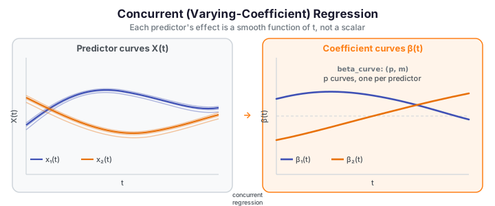
Concurrent regression — also called the varying-coefficient model — extends functional regression by letting each predictor's effect vary smoothly over the domain. Where ordinary linear regression assigns a single scalar coefficient to each predictor, concurrent regression assigns an entire coefficient function \(\beta_k(t)\). At each point \(t\) the model behaves like a local ordinary regression, but the coefficients change fluidly as \(t\) progresses.

fdars.regression.concurrent_regression estimates one smooth coefficient curve per predictor using local kernel regression: the bandwidth controls how quickly the coefficients are allowed to change, and the kernel controls the weighting of neighboring time points.

Concurrent (Varying-Coefficient) Regression — predictor curves and their time-varying coefficient curves

When to use¶

Use concurrent regression when both your predictor and your response are functional (observed on the same grid) and you suspect that the predictor's influence on the response changes at the same point in time — that is, \(X_i(t)\) predicts \(Y_i(t)\) locally without lag or cross-temporal borrowing.

Method	`fdars` function	Response type	Effect structure
Concurrent regression	`concurrent_regression`	functional	\(X(t)\) affects \(Y(t)\) at the same \(t\) — varying coefficient
Function-on-function	`fof_regression`	functional	\(X(t)\) affects \(Y(s)\) for all \(s\) via a global β surface
Scalar-on-function	`fregre_lm` / `fregre_np`	scalar	functional predictor maps to a single number

Quick rule: start with concurrent regression when the physical mechanism is simultaneous (e.g. speed at time \(t\) predicts acceleration at time \(t\), or a temperature curve predicts a precipitation curve at the same day). Switch to function-on-function regression when you expect cross-temporal effects (the predictor at \(t_1\) influences the response at a different \(t_2\)). Use scalar-on-function regression when your response is a single number, not a curve.

Same-grid requirement

Concurrent regression requires that all predictor matrices and the response matrix share the same evaluation grid — same \(n\) observations, same \(m\) grid points. If your predictor and response are observed at different grids, align or interpolate them first.

Theory¶

Given \(p\) functional predictors \(X^{(1)}(t), \dots, X^{(p)}(t)\) and a functional response \(Y(t)\), all observed at the same \(m\) grid points for \(n\) subjects, the model is

\[ Y_i(t) \;=\; \beta_0(t) \;+\; \sum_{k=1}^{p} \beta_k(t)\,X_i^{(k)}(t) \;+\; \varepsilon_i(t), \]

where \(\beta_0(t)\) is a time-varying intercept, \(\beta_1(t), \dots, \beta_p(t)\) are time-varying coefficient functions, and \(\varepsilon_i(t)\) is a zero-mean error process. At each grid point \(t_j\) the function solves a weighted least-squares system with kernel weights centred at \(t_j\):

\[ K_h(t_j - t_s) \;=\; K\!\left(\frac{t_j - t_s}{h}\right), \]

where \(h\) is the bandwidth and \(K\) is the chosen kernel ("gaussian", "epanechnikov", or "tricube"). The resulting \(\hat\beta(t)\) is a smooth estimate of how the coefficient evolves over the domain.

Parameters

Parameter	Type	Default	Description
`predictors`	`list[ndarray (n, m)]`	—	List of \(p\) predictor matrices; each row is one subject's curve
`response`	`ndarray (n, m)`	—	Functional response matrix
`argvals`	`ndarray (m,)` or `None`	`None`	Evaluation grid; `None` → uniform grid on \([0, 1]\)
`bandwidth`	`float`	`0.2`	Kernel bandwidth; must be positive
`kernel`	`str`	`"gaussian"`	Kernel: `"gaussian"`, `"epanechnikov"`, or `"tricube"`

Returns a dict:

Key	Shape	Description
`"beta_curve"`	`(p, m)`	Time-varying coefficient curves — one row per predictor
`"intercept"`	`(m,)`	Time-varying intercept function \(\hat\beta_0(t)\)
`"fitted"`	`(n, m)`	Fitted response curves \(\hat Y_i(t)\)
`"residuals"`	`(n, m)`	Residual curves \(Y_i(t) - \hat Y_i(t)\)
`"argvals"`	`(m,)`	Evaluation grid used (echoed back)

beta_curve shape: (p, m) — predictors × grid

res["beta_curve"] has shape (p, m), where p = len(predictors) and m is the number of grid points. This is not (n, m) — confusing the two is the most common transposition error when working with this function. Row k of beta_curve is the coefficient curve for the k-th predictor, evaluated at every grid point.

1. Fitting the concurrent model¶

The code block below fits a two-predictor concurrent model on synthetic data and visualises the estimated coefficient curves.

import numpy as np
from docs_fig import fig, render, fast
import fdars.regression as reg

rng = np.random.default_rng(0)
n, m = 20, 50
t = np.linspace(0, 1, m)
# Two synthetic predictor curves + a response
x1 = np.array([np.sin(2 * np.pi * t) + rng.normal(0, 0.1, m) for _ in range(n)])
x2 = np.array([np.cos(2 * np.pi * t) + rng.normal(0, 0.1, m) for _ in range(n)])
y  = x1 * np.sin(2 * np.pi * t) + x2 * 0.5 + rng.normal(0, 0.05, (n, m))

res = reg.concurrent_regression([x1, x2], y, t)
beta = np.asarray(res["beta_curve"])  # shape (2, m) — p=2 predictors

f, ax = fig(figsize=(8.0, 3.8))
ax.plot(t, beta[0], color="#3f51b5", lw=2.2, label="β₁(t) — sin predictor")
ax.plot(t, beta[1], color="#e8710a", lw=2.2, label="β₂(t) — cos predictor")
ax.set(title="Concurrent regression — estimated coefficient curves",
       xlabel="t", ylabel="β(t)")
ax.legend(fontsize=9)
print(render(f))
print(f"beta_curve shape: {beta.shape}  (p=2 predictors × m={m} grid points)")
print("FDARS_FENCE_OK")

beta_curve shape: (2, 50) (p=2 predictors × m=50 grid points) FDARS_FENCE_OK

2. Out-of-sample prediction¶

There is no dedicated predict function for concurrent regression in fdars. Prediction on new predictor curves is straightforward matrix algebra on the returned beta_curve and intercept:

\[ \hat{Y}_{new}(t) \;=\; \hat\beta_0(t) \;+\; \sum_{k=1}^{p} \hat\beta_k(t)\,X_{new}^{(k)}(t) \]

Each term is an element-wise product between the coefficient row beta_curve[k, :] (shape (m,)) and the new predictor curve x_k_new (shape (m,)).

import numpy as np
from fdars.regression import concurrent_regression

rng = np.random.default_rng(3)
n, m = 20, 40
t = np.linspace(0, 1, m)

# Fit on training data
x1 = np.array([np.sin(2 * np.pi * t) + rng.normal(0, 0.1, m) for _ in range(n)])
y  = x1 * np.sin(np.pi * t) + rng.normal(0, 0.05, (n, m))

res = concurrent_regression([x1], y, t)
beta = np.asarray(res["beta_curve"])   # shape (1, m) — p=1 predictor
intercept = np.asarray(res["intercept"])  # shape (m,)

# Manual prediction on a new predictor curve (manual formula — no predict function):
x_new = np.sin(2 * np.pi * t + 0.5)            # shape (m,)
y_pred = intercept + beta[0] * x_new            # shape (m,)

print(f"beta_curve shape: {beta.shape}  (p=1 predictor × m={m} grid points)")
print(f"y_pred shape:     {y_pred.shape}")
print(f"y_pred[0:3]:      {y_pred[:3].round(4)}")
print("FDARS_FENCE_OK")

beta_curve shape: (1, 40) (p=1 predictor × m=40 grid points) y_pred shape: (40,) y_pred[0:3]: [0.0491 0.0959 0.1564] FDARS_FENCE_OK

Generalising to p predictors

For \(p > 1\) predictors, sum over all rows of beta_curve:

y_pred = intercept + sum(
    beta[k] * new_predictors[k] for k in range(p)
)

where new_predictors is a list of new predictor curves, each of shape (m,).

3. Bandwidth selection and Caveats¶

Bandwidth selection¶

The bandwidth h is the most consequential tuning choice. There is no built-in cross-validation in concurrent_regression — the user supplies the bandwidth directly.

No built-in bandwidth CV

Unlike scalar-on-function regression (fregre_np_cv), the concurrent model has no built-in cross-validation helper for automatic bandwidth selection. The bandwidth must be chosen manually. The example below shows a minimal leave-one-out style CV loop over candidate bandwidths using held-out prediction MSE — this pattern should be adapted to your data.

Bandwidth trades bias for variance

Small bandwidth (e.g. bandwidth=0.05): the kernel weights few neighbours at each \(t\), so the estimated \(\hat\beta(t)\) tracks local fluctuations closely — resulting in wiggly, high-variance coefficient curves. On small samples this produces noisy estimates that are hard to interpret.
Large bandwidth (e.g. bandwidth=0.5): the kernel pools many neighbours, smoothing over local structure — resulting in over-smoothed, biased estimates that miss true variation in \(\beta(t)\).
Practical starting point: try bandwidth=0.2 (the default) on a normalised argvals grid and inspect the shape of res["beta_curve"]. If the curves look spiky, widen; if they look flat when you expect variation, narrow.

The fence below shows a manual bandwidth search using held-out prediction MSE:

import numpy as np
from fdars.regression import concurrent_regression

rng = np.random.default_rng(7)
n, m = 24, 30
t = np.linspace(0, 1, m)

# Simulate data: beta_true(t) = sin(pi*t)
x1 = np.array([np.sin(2 * np.pi * t) + rng.normal(0, 0.15, m) for _ in range(n)])
y  = x1 * np.sin(np.pi * t) + rng.normal(0, 0.08, (n, m))

# Hold out the last 4 observations for validation
n_train = n - 4
x_train, y_train = x1[:n_train], y[:n_train]
x_val,   y_val   = x1[n_train:], y[n_train:]

candidates = [0.05, 0.10, 0.20, 0.35, 0.50]
mse_scores = []
for bw in candidates:
    res = concurrent_regression([x_train], y_train, t, bandwidth=bw)
    beta = np.asarray(res["beta_curve"])       # (1, m)
    intercept = np.asarray(res["intercept"])   # (m,)
    # Predict on validation set — manual formula (no built-in predict)
    y_hat = intercept[None, :] + x_val * beta[0]  # (4, m)
    mse = float(np.mean((y_val - y_hat) ** 2))
    mse_scores.append(mse)

best_bw = candidates[int(np.argmin(mse_scores))]
print(f"Candidate bandwidths: {candidates}")
print(f"Validation MSE:       {[round(v, 5) for v in mse_scores]}")
print(f"Best bandwidth:       {best_bw}")
print("FDARS_FENCE_OK")

Candidate bandwidths: [0.05, 0.1, 0.2, 0.35, 0.5] Validation MSE: [0.00899, 0.00954, 0.01433, 0.02105, 0.02475] Best bandwidth: 0.05 FDARS_FENCE_OK

Kernel choice¶

The three kernels differ in their support and decay:

Kernel	Support	Decay	When to prefer
`"gaussian"` (default)	infinite (global)	exponential	Smooth data; all observations contribute with decaying weight
`"epanechnikov"`	compact \([\!-1, 1\!]\)	quadratic	Faster computation; observations beyond bandwidth contribute nothing
`"tricube"`	compact \([\!-1, 1\!]\)	cubic	Similar to Epanechnikov; slightly smoother drop-off

For most functional datasets with smooth \(\beta(t)\), the choice of kernel has less impact than the choice of bandwidth. Start with "gaussian".

Model scope: local-at-each-t, not global¶

Concurrent regression is a varying-coefficient (local) model — it does not fit a single global relationship between predictor and response. At each grid point \(t_j\) it runs an independent weighted regression using only the kernel-weighted neighbourhood of \(t_j\). This means:

The model can capture coefficient functions that reverse sign or change shape over the domain.
It cannot borrow information across widely separated regions of \(t\) (unlike a basis-regression approach).
Residuals \(\varepsilon_i(t)\) are not assumed uncorrelated across \(t\) — the model makes no statement about temporal dependence of errors.

References¶

Hastie, T., and Tibshirani, R. (1993). "Varying-coefficient models." Journal of the Royal Statistical Society, Series B, 55(4), 757–796. — foundational paper on the varying-coefficient model.
Fan, J., and Zhang, W. (1999). "Statistical estimation in varying coefficient models." Annals of Statistics, 27(5), 1491–1518. — local polynomial estimation of time-varying coefficients.
Ramsay, J. O., and Silverman, B. W. (2005). Functional Data Analysis, 2nd ed. Springer. — Chapter 14: concurrent regression and the functional linear model.