Andrews Wine: Outlier Detection

Dataset: UCI Wine — 13 chemical measurements for 178 wines from three Piedmont cultivars (Barolo, Grignolino, Barbera), encoded as Andrews curves so that multivariate outlier detection can run through functional tools.

A wine is a multivariate outlier if its combination of 13 measurements is atypical — not necessarily extreme in any single column, but unusual as a whole. Detecting that directly in 13-D is awkward. Once each wine is an Andrews curve, though, "atypical row" becomes "atypical curve", and fdars offers several robust functional outlier detectors. Each standardized row \(x = (x_1, \dots, x_p)\) becomes the Andrews curve

\[ f_x(t) = \frac{x_1}{\sqrt{2}} + x_2\sin t + x_3\cos t + x_4\sin 2t + x_5\cos 2t + \cdots, \qquad t \in [-\pi, \pi]. \]

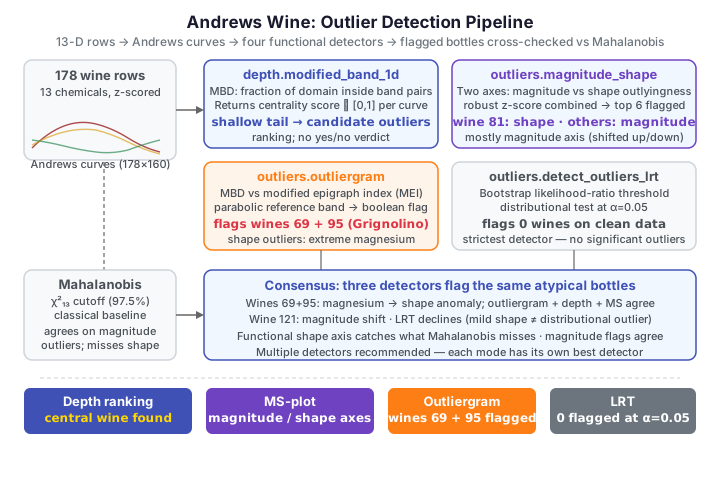
Because the sine/cosine basis is orthogonal on \([-\pi,\pi]\), Parseval's identity gives \(\lVert f_x - f_y\rVert_{L^2}^2 = \pi\,\lVert x - y\rVert_2^2\), so the transform preserves \(L^2\) distances up to the constant \(\sqrt{\pi}\): a curve that is central among the curves corresponds to a wine that is central among the rows. This page runs functional depth, magnitude–shape analysis, the outliergram, and a likelihood-ratio test on the wine curves, cross-checks what they flag, digs into the individual flagged bottles, and finally pits the whole functional pipeline against a classical Mahalanobis baseline.

No andrews binding in fdars

The transform is the same numpy helper introduced on the intro page; fdars handles everything after the curves exist. We z-score the 13 columns before transforming so no single feature dominates the curve.

Depth ranks wines by centrality

Functional depth scores each curve by how central it is within the sample — high depth is typical, low depth is outlying. We use modified_band_1d from fdars.depth, which computes the modified band depth of every curve against the whole set. For a sample of \(n\) curves it averages, over all \(\binom{n}{2}\) pairs, the fraction of the domain on which curve \(f_x\) lies between the pair:

\[ \mathrm{MBD}(f_x) = \binom{n}{2}^{-1} \sum_{i<j} \frac{\lambda\bigl\{ t : \min(f_i,f_j)(t) \le f_x(t) \le \max(f_i,f_j)(t) \bigr\}} {\lambda([-\pi,\pi])}, \]

where \(\lambda\) is Lebesgue measure. A curve threaded through the middle of many bands scores near \(1\); an edge curve scores near \(0\).

import numpy as np
from docs_fig import fig, render
from docs_data import load_wine
from fdars.depth import modified_band_1d

def andrews_curves(features, t):
    features = np.asarray(features, float)
    n, p = features.shape
    out = np.full((n, t.size), features[:, [0]] / np.sqrt(2.0))
    for j in range(1, p):
        harmonic = (j + 1) // 2
        term = np.sin if j % 2 == 1 else np.cos
        out = out + features[:, [j]] * term(harmonic * t)
    return out

names, X, meta = load_wine()
Xz = (X - X.mean(0)) / X.std(0)
t = np.linspace(-np.pi, np.pi, 160)
curves = andrews_curves(Xz, t)

depth = np.asarray(modified_band_1d(curves, curves))
order = np.argsort(depth)                       # shallow (outlying) first
rng_d = np.ptp(depth) + 1e-9

f, ax = fig()
for i in order:                                 # faint = shallow
    ax.plot(t, curves[i], color="#3f51b5", lw=1.0,
            alpha=0.12 + 0.75 * (depth[i] - depth.min()) / rng_d)
ax.plot(t, curves[order[-1]], color="#198754", lw=2.4, label="deepest (typical)")
ax.plot(t, curves[order[0]],  color="#dc3545", lw=2.4, label="shallowest")
ax.set(title="Modified band depth of the wine Andrews curves",
       xlabel="t", ylabel=r"$f_x(t)$")
ax.legend()
print(render(f))

The deepest curve is a thoroughly ordinary wine; the shallowest (red) rides the edge of the bundle. Depth gives a ranking, not a yes/no verdict — for a decision rule we turn to the magnitude–shape plot.

Magnitude–shape: two axes of "unusual"

An outlying curve can be unusual in magnitude (shifted up or down) or in shape (wiggling differently), and these call for different explanations. fdars.outliers.magnitude_shape returns a magnitude outlyingness and a shape outlyingness per curve; plotting one against the other separates the two failure modes.

import numpy as np
from docs_fig import fig, render
from docs_data import load_wine
from fdars.outliers import magnitude_shape

def andrews_curves(features, t):
    features = np.asarray(features, float)
    n, p = features.shape
    out = np.full((n, t.size), features[:, [0]] / np.sqrt(2.0))
    for j in range(1, p):
        harmonic = (j + 1) // 2
        term = np.sin if j % 2 == 1 else np.cos
        out = out + features[:, [j]] * term(harmonic * t)
    return out

names, X, meta = load_wine()
cultivar = meta["cultivar"].to_numpy()
Xz = (X - X.mean(0)) / X.std(0)
t = np.linspace(-np.pi, np.pi, 160)
curves = andrews_curves(Xz, t)

ms = magnitude_shape(curves)
mag = np.asarray(ms["magnitude"])
shp = np.asarray(ms["shape"])

# robust (median / MAD) combined score to rank the most extreme wines
def z(v):
    med = np.median(v)
    mad = np.median(np.abs(v - med)) * 1.4826 + 1e-9
    return (v - med) / mad
score = np.hypot(z(mag), z(shp))
flag = np.argsort(score)[-6:]                   # 6 most extreme

palette = {1: "#3f51b5", 2: "#e8710a", 3: "#198754"}
f, ax = fig()
ax.scatter(mag, shp, c=[palette[c] for c in cultivar], s=30,
           alpha=0.7, edgecolor="white", linewidth=0.4)
ax.scatter(mag[flag], shp[flag], facecolor="none", edgecolor="#dc3545",
           s=140, linewidth=1.8, label="6 most extreme")
for i in flag:
    ax.annotate(str(i), (mag[i], shp[i]), fontsize=8,
                xytext=(4, 3), textcoords="offset points")
ax.set(title="Magnitude–shape plot of the wine curves",
       xlabel="magnitude outlyingness", ylabel="shape outlyingness")
ax.legend()
print(render(f))

Most wines cluster in a dense blob; the flagged points sit far out on the magnitude axis (with one shape extreme, wine 81), meaning they mostly sit unusually high or low overall while one bends differently from the crowd. The colours show these extreme wines are not confined to one cultivar.

The outliergram: a built-in decision rule

The outliergram plots each curve's modified band depth against its modified epigraph index and derives a parabolic reference region; curves that fall below it are flagged as shape outliers. Unlike the magnitude–shape score above, it returns an explicit boolean flag, so it makes the actual call.

import numpy as np
from docs_fig import fig, render
from docs_data import load_wine
from fdars.outliers import outliergram

def andrews_curves(features, t):
    features = np.asarray(features, float)
    n, p = features.shape
    out = np.full((n, t.size), features[:, [0]] / np.sqrt(2.0))
    for j in range(1, p):
        harmonic = (j + 1) // 2
        term = np.sin if j % 2 == 1 else np.cos
        out = out + features[:, [j]] * term(harmonic * t)
    return out

names, X, meta = load_wine()
cultivar = meta["cultivar"].to_numpy()
Xz = (X - X.mean(0)) / X.std(0)
t = np.linspace(-np.pi, np.pi, 160)
curves = andrews_curves(Xz, t)

og = outliergram(curves)
mei = np.asarray(og["mei"])
mbd = np.asarray(og["mbd"])
flagged = np.where(np.asarray(og["outliers"], dtype=bool))[0]   # indices of flagged curves

f, (axL, axR) = fig(ncols=2, figsize=(9.2, 3.6))
axL.scatter(mei, mbd, color="#3f51b5", s=26, alpha=0.7, edgecolor="white")
if flagged.size:
    axL.scatter(mei[flagged], mbd[flagged], color="#dc3545", s=60,
                label="flagged", zorder=3)
    axL.legend()
axL.set(title="Outliergram", xlabel="modified epigraph index",
        ylabel="modified band depth")

for i in range(curves.shape[0]):
    axR.plot(t, curves[i], color="#c9ccd6", lw=0.7, alpha=0.5)
for i in flagged:
    axR.plot(t, curves[i], color="#dc3545", lw=2.2, label=f"wine {i}")
axR.set(title=f"{flagged.size} outlying wines highlighted",
        xlabel="t", ylabel=r"$f_x(t)$")
if flagged.size:
    axR.legend(fontsize=8)
print(render(f))

print("outliergram flags wines:", flagged.tolist(),
      "— cultivars:", [int(cultivar[i]) for i in flagged])

outliergram flags wines: [69, 95] — cultivars: [2, 2]

The left panel shows the flagged curves falling below the parabolic band the outliergram fits between epigraph index and band depth; the right panel redraws those same wines in red against the faded crowd, confirming they weave rather than merely shift.

outliergram(...)["outliers"] is a boolean mask, not indices

The key returns a length-\(n\) boolean array (one flag per curve), so it must be converted with np.where(mask)[0] before it can index into mei, mbd or curves. Passing the raw 0/1 array as an index silently plots the wrong (0th and 1st) curves — a subtle trap worth flagging.

The outliergram singles out two Grignolino wines (69 and 95 on the 0-based grid). Both are extreme in magnesium: wine 69 has \(z \approx +3.6\) and wine 95 \(z \approx +4.4\), and both dip and rise unusually relative to the crowd — genuine shape anomalies rather than mere level shifts. Reassuringly, these are the same two curves that sat lowest on the depth ranking and furthest out on the magnitude–shape plot: three different detectors agreeing on the same handful of atypical bottles.

Validation — the flagged pair and the Parseval identity

Two ground-truth checks anchor this page. (1) The outliergram must flag exactly wines 69 and 95 — the pair named in the prose. (2) The Andrews transform is a Parseval isometry: on \(t \in [-\pi, \pi]\) the \(L^2\) distance between two wine curves equals \(\sqrt{\pi}\) times the Euclidean distance between the standardized rows, so a curve central among curves is a wine central among rows. We assert the ratio equals \(\sqrt{\pi}\) to \(10^{-6}\) (evaluated on a fine grid where the 13-harmonic curves are fully resolved).

import numpy as np
from docs_data import load_wine
from fdars.outliers import outliergram

def andrews_curves(features, t):
    features = np.asarray(features, float)
    n, p = features.shape
    out = np.full((n, t.size), features[:, [0]] / np.sqrt(2.0))
    for j in range(1, p):
        harmonic = (j + 1) // 2
        term = np.sin if j % 2 == 1 else np.cos
        out = out + features[:, [j]] * term(harmonic * t)
    return out

names, X, meta = load_wine()
Xz = (X - X.mean(0)) / X.std(0)

# (1) outliergram flags exactly the pair the prose names
t = np.linspace(-np.pi, np.pi, 160)
curves = andrews_curves(Xz, t)
flagged = np.where(np.asarray(outliergram(curves)["outliers"], dtype=bool))[0]
assert flagged.tolist() == [69, 95], flagged.tolist()

# (2) Parseval: L2 curve distance == sqrt(pi) * Euclidean row distance
tf = np.linspace(-np.pi, np.pi, 4000)          # fine grid -> exact isometry
cf = andrews_curves(Xz, tf)
rng = np.random.default_rng(0)
ratios = []
for _ in range(500):
    i, j = rng.integers(0, len(cf), 2)
    if i == j:
        continue
    l2 = np.sqrt(np.trapezoid((cf[i] - cf[j]) ** 2, tf))
    ratios.append(l2 / np.linalg.norm(Xz[i] - Xz[j]))
ratios = np.array(ratios)
assert np.allclose(ratios, np.sqrt(np.pi), atol=1e-6), (ratios.min(), ratios.max())
print(f"outliergram flags {flagged.tolist()}  (expected [69, 95])")
print(f"L2/Euclidean ratio = {ratios.mean():.9f}  vs  sqrt(pi) = {np.sqrt(np.pi):.9f}")

outliergram flags [69, 95] (expected [69, 95]) L2/Euclidean ratio = 1.772453851 vs sqrt(pi) = 1.772453851

Both assertions pass: the detector reproduces the named pair, and the distance identity holds to machine precision — confirming the functional outlier verdict transfers back to the original 13-D rows without distortion.

A likelihood-ratio test for outliers

detect_outliers_lrt takes a more formal, hypothesis-testing route: it bootstraps a null distribution and flags curves whose likelihood-ratio statistic exceeds a data-driven threshold at level alpha.

import numpy as np
from docs_fig import fig, render
from docs_data import load_wine
from fdars.outliers import detect_outliers_lrt

def andrews_curves(features, t):
    features = np.asarray(features, float)
    n, p = features.shape
    out = np.full((n, t.size), features[:, [0]] / np.sqrt(2.0))
    for j in range(1, p):
        harmonic = (j + 1) // 2
        term = np.sin if j % 2 == 1 else np.cos
        out = out + features[:, [j]] * term(harmonic * t)
    return out

names, X, meta = load_wine()
Xz = (X - X.mean(0)) / X.std(0)
t = np.linspace(-np.pi, np.pi, 160)
curves = andrews_curves(Xz, t)

res = detect_outliers_lrt(curves, alpha=0.05, n_bootstrap=200)
mask = np.asarray(res["outliers"], dtype=bool)
n_flag = int(mask.sum())

f, ax = fig()
for i in range(curves.shape[0]):
    ax.plot(t, curves[i], color="#c9ccd6", lw=0.7, alpha=0.5)
for i in np.where(mask)[0]:
    ax.plot(t, curves[i], color="#dc3545", lw=2.2)
title = (f"LRT flags {n_flag} wines (threshold {res['threshold']:.2f})"
         if n_flag else
         f"LRT flags no wines at α=0.05 (threshold {res['threshold']:.2f})")
ax.set(title=title, xlabel="t", ylabel=r"$f_x(t)$")
print(render(f))

The plot stays uniformly grey: no curve crosses the bootstrapped threshold, so the strictest of our four detectors declines to flag anything on this clean, standardized data set.

A conservative test on a clean data set

On these curves detect_outliers_lrt flags no wines at \(\alpha = 0.05\): the wine measurements are genuinely well-behaved once standardized, so no curve is extreme enough to reject the null of "same distribution". That is the honest result, not a failure — the LRT is a stricter, distributional test than the depth-based outliergram, which flags borderline shape anomalies that the LRT does not consider significant. When detectors disagree like this, the disagreement itself is informative: the flagged wines are mildly unusual in shape but not distributional outliers.

Case studies: what makes the flagged wines unusual

Because the Andrews transform is an isometry, a flagged curve points straight back to a flagged wine whose chemistry we can read off. The three most-extreme wines, ranked by a robust magnitude–shape score, tell three different stories.

import numpy as np
from docs_fig import fig, render
from docs_data import load_wine
from fdars.outliers import magnitude_shape

def andrews_curves(features, t):
    features = np.asarray(features, float)
    n, p = features.shape
    out = np.full((n, t.size), features[:, [0]] / np.sqrt(2.0))
    for j in range(1, p):
        harmonic = (j + 1) // 2
        term = np.sin if j % 2 == 1 else np.cos
        out = out + features[:, [j]] * term(harmonic * t)
    return out

names, X, meta = load_wine()
cultivar = meta["cultivar"].to_numpy()
labels = {1: "Barolo", 2: "Grignolino", 3: "Barbera"}
Xz = (X - X.mean(0)) / X.std(0)
t = np.linspace(-np.pi, np.pi, 160)
curves = andrews_curves(Xz, t)

ms = magnitude_shape(curves)
def z(v):
    med = np.median(v); mad = np.median(np.abs(v - med)) * 1.4826 + 1e-9
    return (v - med) / mad
score = np.hypot(z(np.asarray(ms["magnitude"])), z(np.asarray(ms["shape"])))
cases = np.argsort(score)[-3:][::-1]           # 3 most extreme wines

f, axes = fig(ncols=3, figsize=(10.5, 3.4), sharey=True)
for ax, i in zip(axes, cases):
    c = cultivar[i]
    same = np.where(cultivar == c)[0]
    ax.plot(t, curves[same].T, color="#c9ccd6", lw=0.6, alpha=0.5)
    ax.plot(t, curves[i], color="#dc3545", lw=2.2)
    # within-cultivar z-scores to name the culprit chemicals
    cv = Xz[same]
    dev = (Xz[i] - cv.mean(0)) / cv.std(0)
    top = np.argsort(-np.abs(dev))[:2]
    culprit = ", ".join(f"{names[j]} ({dev[j]:+.1f})" for j in top)
    ax.set(title=f"wine {i} — {labels[c]}", xlabel="t")
    ax.text(0.5, 0.02, culprit, transform=ax.transAxes, fontsize=7.5,
            ha="center", va="bottom", color="#333")
axes[0].set(ylabel=r"$f_x(t)$")
print(render(f))

for i in cases:
    c = cultivar[i]; same = np.where(cultivar == c)[0]
    dev = (Xz[i] - Xz[same].mean(0)) / Xz[same].std(0)
    top = np.argsort(-np.abs(dev))[:3]
    print(f"wine {i:3d} ({labels[c]:10s}): " +
          ", ".join(f"{names[j]} z={dev[j]:+.1f} within-cultivar" for j in top))

wine 95 (Grignolino): magnesium z=+4.1 within-cultivar, proanthocyanins z=+2.8 within-cultivar, proline z=+2.7 within-cultivar wine 69 (Grignolino): magnesium z=+3.4 within-cultivar, nonflavanoid_phenols z=-1.8 within-cultivar, ash z=-1.6 within-cultivar wine 121 (Grignolino): flavanoids z=+4.3 within-cultivar, color_intensity z=+3.2 within-cultivar, ash z=+3.1 within-cultivar

All three most-extreme wines are Grignolino, but they are unusual for different reasons:

• Wines 69 and 95 — the pair the outliergram flagged — carry a huge magnesium excess (within-cultivar \(z \approx +3.4\) and \(+4.1\)), wine 95 compounded by high proanthocyanins. Their curves dip and weave through the Grignolino envelope: a shape anomaly a soil-chemistry investigation would chase down, not a measurement slip.
• Wine 121 is the flip side — elevated flavanoids and colour intensity (\(z \approx +4\) and \(+3\)) lift the whole curve, a more magnitude-like signature consistent with an unusually concentrated bottle.

That the functional detectors concentrate on Grignolino is itself informative: it is the largest and most heterogeneous cultivar (widest envelope on the intro page), so its fringes host the wines most easily mistaken for another class. The payoff of the functional view is exactly this — the curves three detectors independently flagged decompose into interpretable, actionable chemistry.

A classical baseline: Mahalanobis distance

Do we need the functional machinery at all, or would a textbook multivariate outlier rule do the same job? The Mahalanobis distance is the standard answer: it measures each wine's distance from the centre in the covariance metric and flags any exceeding a \(\chi^2_{13}\) cutoff at the 97.5% level. We compare its verdict against the union of the functional detectors.

import numpy as np
from scipy.stats import chi2
from docs_fig import fig, render
from docs_data import load_wine
from fdars.depth import modified_band_1d
from fdars.outliers import magnitude_shape, outliergram

def andrews_curves(features, t):
    features = np.asarray(features, float)
    n, p = features.shape
    out = np.full((n, t.size), features[:, [0]] / np.sqrt(2.0))
    for j in range(1, p):
        harmonic = (j + 1) // 2
        term = np.sin if j % 2 == 1 else np.cos
        out = out + features[:, [j]] * term(harmonic * t)
    return out

names, X, meta = load_wine()
Xz = (X - X.mean(0)) / X.std(0)
t = np.linspace(-np.pi, np.pi, 160)
curves = andrews_curves(Xz, t)

# classical Mahalanobis outliers
cov_inv = np.linalg.inv(np.cov(Xz, rowvar=False))
mahal = np.einsum("ij,jk,ik->i", Xz, cov_inv, Xz)
cutoff = chi2.ppf(0.975, df=Xz.shape[1])
mahal_out = set(np.where(mahal > cutoff)[0].tolist())

# functional union (depth-shallow + MS-extreme + outliergram)
depth = np.asarray(modified_band_1d(curves, curves))
shallow = set(np.argsort(depth)[:9].tolist())
ms = magnitude_shape(curves)
def z(v):
    med = np.median(v); mad = np.median(np.abs(v - med)) * 1.4826 + 1e-9
    return (v - med) / mad
ms_score = np.hypot(z(np.asarray(ms["magnitude"])), z(np.asarray(ms["shape"])))
ms_out = set(np.argsort(ms_score)[-6:].tolist())
og_out = set(np.where(np.asarray(outliergram(curves)["outliers"], dtype=bool))[0].tolist())
fda_out = shallow | ms_out | og_out

both = sorted(mahal_out & fda_out)
mahal_only = sorted(mahal_out - fda_out)
fda_only = sorted(fda_out - mahal_out)

f, ax = fig(figsize=(6.4, 4.0))
ax.bar(["both", "Mahalanobis\nonly", "functional\nonly"],
       [len(both), len(mahal_only), len(fda_only)],
       color=["#198754", "#6c757d", "#3f51b5"])
ax.set(title="Mahalanobis vs functional detectors", ylabel="number of wines")
print(render(f))

print("agreed by both:      ", both)
print("Mahalanobis only:    ", mahal_only)
print("functional only:     ", fda_only)

agreed by both: [13, 59, 69, 73, 95, 115, 121, 158] Mahalanobis only: [71, 96, 110, 159] functional only: [14, 81]

The two philosophies substantially agree: a solid core of wines is flagged by both the covariance-based rule and the functional detectors — including the Grignolino magnesium pair and the Barbera colour outlier. Where they differ is instructive. Mahalanobis, being a pure magnitude-in-covariance rule, catches a few extra wines that are far from the centre but ordinary in shape; the functional detectors surface a shape anomaly or two that Mahalanobis misses. The functional pipeline is not merely a re-skin of the classical test — it adds a shape axis of outlyingness the covariance rule cannot see, while recovering essentially the same magnitude outliers.

What the detectors found

Method	Binding	Output	On the wine curves
Modified band depth	depth.modified_band_1d	centrality score per curve	ranking; shallowest wines are borderline
Magnitude–shape	outliers.magnitude_shape	magnitude, shape per curve	extreme wines are shape-unusual
Outliergram	outliers.outliergram	mei, mbd, outliers (bool mask)	flags 2 Grignolino shape outliers (69, 95)
LRT	outliers.detect_outliers_lrt	outliers mask, threshold	none significant at α=0.05
Mahalanobis (classical)	numpy + scipy.stats.chi2	\(\chi^2_{13}\) cutoff	agrees on the magnitude outliers

The picture is consistent: a few wines (the same ones across depth, MS and the outliergram) are mildly atypical in curve shape, but none are strong enough to register as distributional outliers. For a quality-control setting where you expect some bottles to be off-spec, see the QC page, which monitors one cultivar against another with control charts.

See also

• Functional depth — the depth measures used here.
• Andrews Wine intro — the transform and class structure.
• Clustering & variable importance — recovering the cultivars.

References

• Andrews, D.F. (1972). Plots of high-dimensional data. Biometrics 28(1):125-136.
• Lopez-Pintado, S., Romo, J. (2009). On the concept of depth for functional data. JASA 104(486):718-734.
• Arribas-Gil, A., Romo, J. (2014). Shape outlier detection and visualization for functional data: the outliergram. Biostatistics 15(4):603-619.
• Dai, W., Genton, M.G. (2018). Multivariate functional data visualization and outlier detection. JCGS 27(4):923-934.