Elastic FPCA

Ordinary Functional PCA assumes that curves differ only in amplitude -- their height at each fixed time \(t\). Real curves often also differ in phase: the same feature (a peak, a crossing) occurs at different times in different observations. When amplitude and phase variation are entangled, ordinary FPCA wastes components describing the misalignment and the leading eigenfunctions become hard to interpret. Elastic FPCA first separates the two sources of variation using the square-root-slope framework, then runs PCA in the amplitude space, the phase (warping) space, or jointly.

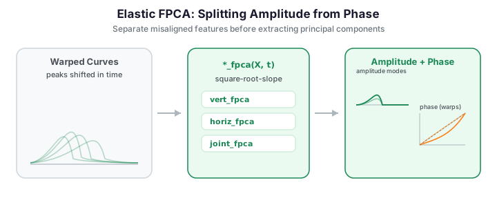
Each bump differs in both its peak height (amplitude) and the horizontal position of its peak (phase). Because the peaks are scattered along the time axis, a pointwise method like ordinary FPCA cannot line them up and would spend components describing the horizontal drift.

Concepts: amplitude and phase

Write each observed curve as a warped version of an underlying template:

\[ X_i(t) = a_i \cdot f\bigl(\gamma_i(t)\bigr) \]

where \(\gamma_i:[0,1]\to[0,1]\) is a monotone increasing warping function (phase) and \(a_i\) scales amplitude. The goal is to decompose the sample into

• an amplitude part -- the aligned curves, all sharing a common time axis, and
• a phase part -- the warping functions \(\gamma_i\) that map each curve onto the template.

The mathematics is cleanest in the square-root-slope function (SRSF) representation. For a curve \(f\) with derivative \(\dot f\),

\[ q(t) = \operatorname{sign}\bigl(\dot f(t)\bigr)\sqrt{\lvert \dot f(t)\rvert}. \]

The SRSF turns the awkward, non-Euclidean geometry of warping into a plain \(L^2\) geometry on the unit Hilbert sphere. The Fisher--Rao distance between two curves, which is invariant to how we parameterize time, then reduces to an \(L^2\) distance between SRSFs after optimal alignment:

\[ d_{\mathrm{FR}}(f_1, f_2) = \inf_{\gamma \in \Gamma}\, \bigl\lVert q_1 - (q_2 \circ \gamma)\sqrt{\dot\gamma}\,\bigr\rVert_2, \]

where \(\Gamma\) is the group of orientation-preserving warps \(\gamma:[0,1]\to[0,1]\) and \((q_2\circ\gamma)\sqrt{\dot\gamma}\) is the SRSF of the warped curve \(f_2\circ\gamma\). fdars exposes the transform and the resulting elastic mean directly:

from fdars.alignment import srsf_transform, karcher_mean

q = srsf_transform(curve, argvals)      # SRSF of a single curve
km = karcher_mean(data, argvals)        # elastic (Karcher) mean + alignment

karcher_mean returns the template and the by-products of alignment:

Key	Shape	Description
mean	(m,)	Elastic (Karcher) mean curve -- the template
mean_srsf	(m,)	SRSF of the template
aligned_data	(n, m)	Each curve warped onto the template (amplitude part)
gammas	(n, m)	Warping functions \(\gamma_i\) (phase part)
n_iter	scalar	Iterations to convergence
converged	bool	Whether the fixed-point iteration converged

The figure below shows the effect of alignment: after warping every curve onto the Karcher mean, the peaks line up and the residual spread is pure amplitude.

import numpy as np
from docs_fig import fig, render
from fdars.alignment import karcher_mean

t = np.linspace(0, 1, 100)
rng = np.random.default_rng(3)
X = np.asarray([
    (1.0 + 0.25 * rng.standard_normal()) *
    np.exp(-((t - (0.5 + 0.12 * rng.standard_normal())) ** 2) / 0.01)
    for _ in range(25)
])

km = karcher_mean(X, t)
aligned = np.asarray(km["aligned_data"])
mean = np.asarray(km["mean"])

f, (a0, a1) = fig(1, 2, figsize=(10, 3.8))
a0.plot(t, X.T, color="#3f51b5", lw=1, alpha=0.4)
a0.set(title="Original (amplitude + phase)", xlabel="t", ylabel="X(t)")
a1.plot(t, aligned.T, color="#198754", lw=1, alpha=0.4)
a1.plot(t, mean, color="#dc3545", lw=2.4, label="Karcher mean")
a1.set(title="Aligned (amplitude only)", xlabel="t", ylabel="X(t)")
a1.legend()
print(render(f))

In the right panel every bump peaks at the same location as the Karcher mean (red): the horizontal scatter of the left panel has been absorbed into the warping functions, leaving only vertical (amplitude) spread. This is exactly the separation elastic FPCA exploits.

Validation: alignment reduces amplitude variance; warps are valid; distances agree

Three properties that alignment must satisfy are asserted below. (1) Warping the curves onto the template collapses the cross-sectional (pointwise) variance: the integrated pointwise variance of the aligned curves is strictly smaller than that of the originals, because the horizontal spread has been removed. (2) Every warping function \(\gamma_i\) is a valid element of the warping group \(\Gamma\) -- monotone non-decreasing with \(\gamma(0)=0\), \(\gamma(1)=1\), and range in \([0,1]\). (3) The Fisher-Rao amplitude distance equals the elastic distance to machine precision, since after optimal alignment they are the same \(L^2\) SRSF distance. All checks pass.

import numpy as np
from fdars.alignment import karcher_mean, amplitude_distance, elastic_distance

t = np.linspace(0, 1, 100)
rng = np.random.default_rng(3)
X = np.asarray([
    (1.0 + 0.25 * rng.standard_normal()) *
    np.exp(-((t - (0.5 + 0.12 * rng.standard_normal())) ** 2) / 0.01)
    for _ in range(25)
])

km = karcher_mean(X, t)
aligned = np.asarray(km["aligned_data"])
gammas = np.asarray(km["gammas"])

# (1) Alignment reduces the integrated cross-sectional variance.
var_orig = X.var(axis=0).mean()
var_aligned = aligned.var(axis=0).mean()
assert var_aligned < var_orig, (var_aligned, var_orig)
print(f"cross-sectional variance: {var_orig:.4f} -> {var_aligned:.4f} "
      f"({100 * (1 - var_aligned / var_orig):.0f}% reduction)")

# (2) Warps live in the warping group Gamma: monotone, range [0,1], fixed ends.
assert (np.diff(gammas, axis=1) >= -1e-9).all()               # monotone
assert gammas.min() >= -1e-9 and gammas.max() <= 1 + 1e-9      # range [0,1]
assert np.abs(gammas[:, 0]).max() < 1e-9                       # gamma(0) = 0
assert np.abs(gammas[:, -1] - 1).max() < 1e-9                  # gamma(1) = 1
print("all 25 warps monotone, range [0,1], gamma(0)=0, gamma(1)=1")

# (3) amplitude_distance == elastic_distance (same post-alignment L2 distance).
ad = float(amplitude_distance(X[0], X[1], t))
ed = float(elastic_distance(X[0], X[1], t))
assert abs(ad - ed) < 1e-10, (ad, ed)
print(f"amplitude_distance {ad:.6f} == elastic_distance {ed:.6f} "
      f"(|diff| = {abs(ad - ed):.1e})")

cross-sectional variance: 0.0673 -> 0.0114 (83% reduction) all 25 warps monotone, range [0,1], gamma(0)=0, gamma(1)=1 amplitude_distance 0.315107 == elastic_distance 0.315107 (|diff| = 0.0e+00)

The warping functions \(\gamma_i\) returned in gammas are the phase part -- one monotone map per curve describing how its time axis was stretched to reach the template. A warp bowing above the diagonal advances the peak, one below it delays the peak; the spread of the warps around the identity is the amount of phase variation in the sample.

import numpy as np
from docs_fig import fig, render
from fdars.alignment import karcher_mean

t = np.linspace(0, 1, 100)
rng = np.random.default_rng(3)
X = np.asarray([
    (1.0 + 0.25 * rng.standard_normal()) *
    np.exp(-((t - (0.5 + 0.12 * rng.standard_normal())) ** 2) / 0.01)
    for _ in range(25)
])

km = karcher_mean(X, t)
gammas = np.asarray(km["gammas"])

f, ax = fig()
ax.plot(t, gammas.T, color="#6f42c1", lw=1, alpha=0.5)
ax.plot([0, 1], [0, 1], color="#dc3545", lw=1.6, ls="--", label="identity (no warp)")
ax.set(title="Warping functions $\\gamma_i$ (phase information)",
       xlabel="t", ylabel=r"$\gamma(t)$")
ax.legend()
print(render(f))

The warps fan out around the diagonal identity (red dashed): curves whose \(\gamma\) bows above the diagonal had their peak advanced during alignment, those below had it delayed. The width of this fan is the amount of phase variation in the sample.

The three elastic FPCA variants

Once amplitude and phase are separated, fdars.alignment provides three PCA routines. They share a signature and each return a dict.

from fdars.alignment import vert_fpca, horiz_fpca, joint_fpca

amp   = vert_fpca(data, argvals, n_comp=3)   # amplitude-space PCA
phase = horiz_fpca(data, argvals, n_comp=3)  # phase / warping-space PCA
both  = joint_fpca(data, argvals, n_comp=3)  # joint amplitude-phase PCA

Parameter	Type	Default	Description
data	np.ndarray (n, m)	--	Discretized curves
argvals	np.ndarray (m,)	--	Common evaluation grid
n_comp	int	3	Number of components to retain
lambda_	float	0.0	Warping-smoothness penalty used during alignment
max_iter	int	20	Max alignment iterations
tol	float	1e-4	Convergence tolerance

Vertical (amplitude) FPCA

vert_fpca runs PCA on the aligned curves, so its components describe amplitude variation with phase removed. Its returned dict contains:

Key	Shape	Description
scores	(n, n_comp)	Amplitude scores
eigenfunctions_f	(n_comp, m)	Eigenfunctions in the original (function) space
eigenfunctions_q	(n_comp, m+1)	Eigenfunctions in SRSF space
eigenvalues	(n_comp,)	Variance per component
cumulative_variance	(n_comp,)	Cumulative variance fraction
mean_q	(m+1,)	SRSF-space mean

The modes of amplitude variation, \(\hat\mu \pm 2\sqrt{\lambda_k}\,\phi_k\), are plotted in the original function space via eigenfunctions_f:

import numpy as np
from docs_fig import fig, render
from fdars.alignment import vert_fpca, karcher_mean

t = np.linspace(0, 1, 100)
rng = np.random.default_rng(3)
X = np.asarray([
    (1.0 + 0.25 * rng.standard_normal()) *
    np.exp(-((t - (0.5 + 0.12 * rng.standard_normal())) ** 2) / 0.01)
    for _ in range(25)
])

amp = vert_fpca(X, t, n_comp=3)
phi = np.asarray(amp["eigenfunctions_f"])         # (n_comp, m)
lam = np.asarray(amp["eigenvalues"])
cumvar = np.asarray(amp["cumulative_variance"])
mean = np.asarray(karcher_mean(X, t)["mean"])     # template in function space

# The function-space eigenfunctions carry a constant (DC) offset from the SRSF
# inversion; subtract each one's flat-region level so the mode oscillates
# around the mean instead of sitting on a pedestal.
phi = phi - np.median(phi, axis=1, keepdims=True)

f, ax = fig()
ax.plot(t, mean, color="#6c757d", lw=1.6, ls="--", label="amplitude mean")
colors = ["#3f51b5", "#e8710a"]
for k in range(2):
    c = 2 * np.sqrt(lam[k])
    ax.plot(t, mean + c * phi[k], color=colors[k], lw=1.8,
            label=f"mode {k+1} $\\pm$2 SD")
    ax.plot(t, mean - c * phi[k], color=colors[k], lw=1.8, ls=":")
ax.set(title="Amplitude modes of variation (vert_fpca)",
       xlabel="t", ylabel="X(t)")
ax.legend()
print(render(f))

Both modes keep the peak fixed in time and vary only its height and width -- exactly what "amplitude with phase removed" should look like. Mode 1 mainly raises or lowers the whole bump, while mode 2 adjusts its sharpness, and neither shifts the peak sideways.

Horizontal (phase) FPCA

horiz_fpca runs PCA on the warping functions -- the phase. Because warping functions live on a curved space (the space of monotone maps), the PCA operates on their shooting vectors in the tangent space at the identity warp. Its dict adds phase-specific keys:

Key	Shape	Description
scores	(n, n_comp)	Phase scores
eigenfunctions_gam	(n_comp, m)	Warping-function eigen-directions
eigenfunctions_psi	(n_comp, m)	SRSF-of-warping eigen-directions
mean_psi	(m,)	Mean warping SRSF
shooting_vectors	(n, m)	Tangent-space representation of each \(\gamma_i\)

Plotting the warping functions reconstructed from the leading phase component shows how the timing of the feature varies across the sample -- warps bowing above the diagonal advance the peak, those below delay it.

import numpy as np
from docs_fig import fig, render
from fdars.alignment import horiz_fpca

t = np.linspace(0, 1, 100)
rng = np.random.default_rng(3)
X = np.asarray([
    (1.0 + 0.25 * rng.standard_normal()) *
    np.exp(-((t - (0.5 + 0.12 * rng.standard_normal())) ** 2) / 0.01)
    for _ in range(25)
])

phase = horiz_fpca(X, t, n_comp=3)
gam = np.asarray(phase["eigenfunctions_gam"])       # phase eigen-directions
cumvar = np.asarray(phase["cumulative_variance"])

f, ax = fig()
ax.plot([0, 1], [0, 1], color="#6c757d", lw=1.2, ls="--", label="identity warp")
for k in range(3):
    ax.plot(t, gam[k], lw=1.8, label=f"phase dir {k+1}")
ax.set(title="Phase (warping) eigen-directions (horiz_fpca)",
       xlabel="t", ylabel=r"$\gamma(t)$")
ax.legend()
print(render(f))

The leading phase direction departs most from the identity warp, describing the dominant pattern of peak timing across the sample; the higher directions add progressively finer timing adjustments. Together they parameterise when the feature occurs, independently of its height.

Joint FPCA

joint_fpca concatenates the amplitude (SRSF) and phase (shooting-vector) representations into a single vector per curve, then runs one PCA on the stack. Its components capture coupled amplitude-phase variation -- useful when, say, taller peaks also tend to arrive earlier. A scalar balance_c rescales the phase block relative to the amplitude block before the joint SVD, so that neither dominates purely because of its units.

Key	Shape	Description
scores	(n, n_comp)	Joint scores
eigenvalues	(n_comp,)	Variance per joint component
cumulative_variance	(n_comp,)	Cumulative variance fraction
vert_component	(n_comp, m+1)	Amplitude part of each joint mode
horiz_component	(n_comp, m)	Phase part of each joint mode
balance_c	scalar	Amplitude/phase balancing constant

joint_fpca reports a single cumulative-variance curve for the coupled representation. To gauge how much of the sample's total variation is amplitude versus phase, compare the amplitude-space and phase-space eigenvalues directly (from vert_fpca and horiz_fpca). Here we deliberately use a sample with large phase variation (the peak location wanders widely) and only modest amplitude variation, so phase carries roughly half the total variance.

joint_fpca's internal balance

This binding's joint_fpca auto-computes a small balance_c, which down-weights the phase (warping) block relative to the amplitude block before the joint SVD -- so its returned horiz_component energy is near zero and its joint modes essentially track the amplitude modes. To see the genuine amplitude/phase split we therefore read the two eigenvalue spectra from vert_fpca / horiz_fpca rather than the joint horiz_component.

import numpy as np
from docs_fig import fig, render
from fdars.alignment import joint_fpca, vert_fpca, horiz_fpca

t = np.linspace(0, 1, 100)
rng = np.random.default_rng(3)
# Large phase variation (wide range of peak locations), modest amplitude.
X = np.asarray([
    (1.0 + 0.08 * rng.standard_normal()) *
    np.exp(-((t - (0.5 + 0.15 * rng.standard_normal())) ** 2) / (2 * 0.01))
    for _ in range(30)
])

joint = joint_fpca(X, t, n_comp=3)
cumvar = np.asarray(joint["cumulative_variance"])

# Genuine amplitude vs phase split from the two elastic spectra.
amp_ev = np.asarray(vert_fpca(X, t, n_comp=3)["eigenvalues"])
phase_ev = np.asarray(horiz_fpca(X, t, n_comp=3)["eigenvalues"])
amp_share = amp_ev.sum() / (amp_ev.sum() + phase_ev.sum())

f, (a0, a1) = fig(1, 2, figsize=(10, 3.8))
ks = np.arange(1, len(cumvar) + 1)
a0.plot(ks, cumvar, "o-", color="#6f42c1")
a0.set(title="Joint FPCA cumulative variance", xlabel="component",
       ylabel="cumulative variance", ylim=(0, 1.02), xticks=ks)
a1.bar(["amplitude", "phase"], [amp_share, 1 - amp_share],
       color=["#198754", "#6f42c1"])
a1.set(title="Amplitude vs phase share of total variance",
       ylabel="variance fraction", ylim=(0, 1.0))
a1.axhline(0.5, ls="--", color="#6c757d", lw=1)
print(render(f))

With this phase-rich sample the two blocks are near-balanced -- phase accounts for close to half the total variation, exactly the regime where separating amplitude and phase pays off.

Contrast with ordinary FPCA

The payoff of separating amplitude and phase is a more parsimonious decomposition. When curves are misaligned, ordinary FPCA needs several components just to represent the horizontal shifting, so its cumulative-variance curve rises slowly. Amplitude FPCA, operating on aligned curves, concentrates the variance in the first component.

The green amplitude-FPCA curve rises far more steeply than the blue ordinary-FPCA curve, reaching the 95 % line in fewer components. Ordinary FPCA wastes components encoding the horizontal misalignment, whereas aligning first concentrates almost all amplitude variance into the first mode.

When to reach for elastic FPCA

If a functional boxplot or a plot of the raw curves shows features (peaks, zero-crossings) drifting horizontally between observations, ordinary FPCA will mix that phase variation into its amplitude components. Separating the two with vert_fpca / horiz_fpca yields interpretable, low-dimensional summaries of what varies (amplitude) and when it varies (phase).

Related tools

The alignment itself, distances, and boxplots live alongside these routines in fdars.alignment: see karcher_mean, amplitude_distance, phase_distance, and phase_boxplot. For the standard (amplitude-only) decomposition, see Functional PCA.

Which variant, and when

Variant	Use it when you want to understand...	Typical questions
vert_fpca	pure shape variation, timing removed	How do the aligned curves differ in height/shape?
horiz_fpca	pure timing variation	How much, and in what pattern, does the feature drift in time?
joint_fpca	coupled amplitude-phase variation	Do taller peaks tend to arrive earlier? What is the amplitude/phase balance?

Concrete examples: for growth curves, vertical FPCA describes differences in final height and spurt magnitude, while horizontal FPCA describes differences in the timing of the pubertal spurt. For gait or movement data, vertical captures the movement pattern and horizontal the stride timing. For weather curves, vertical captures the shape of the seasonal temperature cycle and horizontal the seasonal shift between stations.

References

• Srivastava, A., Wu, W., Kurtek, S., Klassen, E. and Marron, J.S. (2011). Registration of functional data using Fisher-Rao metric. arXiv:1103.3817.
• Tucker, J.D., Wu, W. and Srivastava, A. (2013). Generative models for functional data using phase and amplitude separation. Computational Statistics & Data Analysis 61, 50-66.
• Srivastava, A. and Klassen, E.P. (2016). Functional and Shape Data Analysis. Springer.
• Ramsay, J.O. and Silverman, B.W. (2005). Functional Data Analysis, 2nd ed. Springer.

API summary

Function	Module	Purpose
srsf_transform(curve, argvals)	fdars.alignment	Square-root-slope transform of one curve
karcher_mean(data, argvals, ...)	fdars.alignment	Elastic template + aligned curves + warps
vert_fpca(data, argvals, n_comp, ...)	fdars.alignment	Amplitude-space FPCA
horiz_fpca(data, argvals, n_comp, ...)	fdars.alignment	Phase (warping)-space FPCA
joint_fpca(data, argvals, n_comp, ...)	fdars.alignment	Joint amplitude-phase FPCA
fpca(data, argvals, n_comp)	fdars.regression	Ordinary (amplitude-only) FPCA