Conformal Prediction for Classification

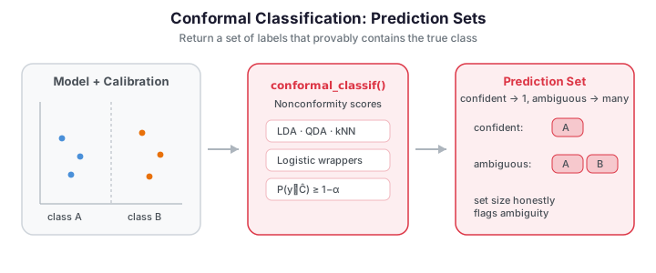
A functional classifier hands you a single predicted label, but that label is a point estimate with no attached reliability. Conformal prediction replaces it with a prediction set — a subset of the classes — that provably contains the true label with a user-chosen probability, using only the mild assumption that the data are exchangeable. When the classifier is confident, the set is a single label; when the curve sits near a decision boundary, the set contains several labels, honestly flagging the ambiguity.

fdars.conformal provides conformal wrappers for functional classifiers: conformal_classif around FPC-based LDA/QDA/kNN, and conformal_logistic / conformal_elastic_logistic around functional logistic regression. All follow the same split-conformal recipe and expose the finite-sample coverage guarantee \(\mathbb{P}(y \in \hat C(x)) \ge 1 - \alpha\).

import numpy as np
from docs_fig import fig, render
from fdars.simulation import simulate
from fdars.conformal import conformal_classif

np.random.seed(1)
t = np.linspace(0, 1, 60)
# two classes with different mean shapes, overlapping fluctuations
Xa = 0.5 * np.asarray(simulate(n=25, argvals=t, n_basis=6, efun_type="fourier", seed=1)) + np.sin(2 * np.pi * t)
Xb = 0.5 * np.asarray(simulate(n=25, argvals=t, n_basis=6, efun_type="fourier", seed=2)) + np.sin(2 * np.pi * t) + 1.0 * t
X = np.vstack([Xa, Xb])
labels = np.r_[np.zeros(25, int), np.ones(25, int)]
perm = np.random.permutation(50)
X, labels = X[perm], labels[perm]
Xtr, ytr, Xte, yte = X[:40], labels[:40], X[40:], labels[40:]

alphas = np.array([0.05, 0.1, 0.15, 0.2, 0.3])
cov, size = [], []
for a in alphas:
    r = conformal_classif(Xtr, ytr, Xte, ncomp=3, classifier="lda",
                          cal_fraction=0.3, alpha=a, seed=1)
    cov.append(r["coverage"])
    size.append(np.mean([len(s) for s in r["prediction_sets"]]))

f, ax = fig()
ax.plot(alphas, cov, "-o", color="#3f51b5", lw=2, label="empirical coverage")
ax.plot(alphas, 1 - alphas, ls="--", color="#6c757d", lw=1.5, label=r"target $1-\alpha$")
ax2 = ax.twinx()
ax2.plot(alphas, size, "-s", color="#e8710a", lw=2, label="mean set size")
ax.set(title="Coverage and set size vs. miscoverage level",
       xlabel=r"$\alpha$", ylabel="coverage")
ax2.set_ylabel("mean prediction-set size")
ax.legend(loc="lower left", fontsize=8)
ax2.legend(loc="upper right", fontsize=8)
print(render(f))

As \(\alpha\) increases the coverage requirement relaxes, and the prediction sets shrink — eventually to single labels. This coverage–informativeness trade-off is the central dial of conformal classification.

Concepts

Split conformal. Reserve a calibration subset from the training data. Fit the base classifier on the rest, then for each calibration point compute a nonconformity score \(s_i\) — how poorly the true label conforms to the classifier's output (e.g. one minus the predicted probability of the true class). Let \(\hat q\) be the \(\lceil(1-\alpha)(n_{\text{cal}}+1)\rceil\)-th smallest score. For a new curve \(x\), the prediction set collects every label whose nonconformity score would be below \(\hat q\):

\[ \hat C(x) = \{\, c : s(x, c) \le \hat q \,\}. \]

Under exchangeability this construction satisfies the marginal coverage guarantee

\[ \mathbb{P}\big(y \in \hat C(x)\big) \ge 1 - \alpha, \]

for any base classifier, with no distributional assumptions — a curve near the boundary simply admits more labels into its set.

Set size	Interpretation
1	Confident, unambiguous prediction
2+ (all classes)	Curve is near a boundary; classifier abstains among these labels
0 (empty)	No label conforms; the curve is atypical of every class (possible outlier)

FPC-based classifiers — conformal_classif

import numpy as np
from fdars.simulation import simulate
from fdars.conformal import conformal_classif

np.random.seed(1)
t = np.linspace(0, 1, 60)
Xa = 0.5 * np.asarray(simulate(n=25, argvals=t, n_basis=6, efun_type="fourier", seed=1)) + np.sin(2 * np.pi * t)
Xb = 0.5 * np.asarray(simulate(n=25, argvals=t, n_basis=6, efun_type="fourier", seed=2)) + np.sin(2 * np.pi * t) + 1.0 * t
X = np.vstack([Xa, Xb])
labels = np.r_[np.zeros(25, int), np.ones(25, int)]
perm = np.random.permutation(50)
X, labels = X[perm], labels[perm]

res = conformal_classif(X[:40], labels[:40], X[40:], ncomp=3,
                        classifier="lda", cal_fraction=0.3, alpha=0.1, seed=1)

print(f"guaranteed coverage: {1 - 0.1:.2f}")
print(f"empirical coverage:  {res['coverage']:.2f}")
print(f"first 5 sets:        {res['prediction_sets'][:5]}")

Parameter	Type	Description
data	ndarray (n, m)	Training functional predictors
labels	ndarray (n,)	Integer class labels
test_data	ndarray (n_test, m)	Curves to predict
ncomp	int	Number of FPC components
classifier	str	Base classifier ("lda", "qda", "knn")
cal_fraction	float	Fraction of training data held for calibration
alpha	float	Miscoverage level (\(1-\alpha\) coverage target)
seed	int	Random seed for the calibration split

Return key	Type	Description
prediction_sets	list[list[int]]	Label set for each test curve
coverage	float	Empirical coverage on the test curves

Logistic classifiers — conformal_logistic

For binary problems, conformal_logistic wraps functional logistic regression the same way. It expects float labels coded 0.0 / 1.0.

import numpy as np
from fdars.conformal import conformal_logistic

y01 = labels.astype(np.float64)                   # 0.0 / 1.0 labels
res = conformal_logistic(X[:40], y01[:40], X[40:], ncomp=3,
                         cal_fraction=0.3, alpha=0.1, seed=1)
sizes = [len(s) for s in res["prediction_sets"]]
print(f"empirical coverage: {res['coverage']:.2f}")
print(f"mean set size:      {np.mean(sizes):.2f}")

For elastic (warping-invariant) logistic classification of shape-driven labels, use conformal_elastic_logistic, which takes the same data, labels, test_data plus an argvals grid and a lambda_ warping-penalty argument.

The distribution of prediction-set sizes shows how often the classifier is decisive versus uncertain at a chosen \(\alpha\):

At the stricter \(\alpha=0.1\) level more curves land in size-2 sets (the classifier hedges to keep its coverage promise), whereas relaxing to \(\alpha=0.3\) pushes most curves into decisive singletons — a direct visual of the coverage-informativeness dial at work.

A three-class example

The two-class demo above keeps things minimal; the more common case has several classes with characteristic shapes. Here class 0 is a distinct, high-amplitude sine — easy to separate — while classes 1 and 2 are both cosine-dominated and differ only by a faint linear drift in class 2, so the 1-vs-2 pair is genuinely confusable. The noise is large enough that individual curves from the two cosine classes overlap heavily.

import numpy as np
from docs_fig import fig, render

np.random.seed(42)
n_per, m = 120, 60
t = np.linspace(0, 1, m)
n = 3 * n_per
X = np.zeros((n, m))
for i in range(n_per):
    X[i] = 1.4 * np.sin(2 * np.pi * t) + 0.5 * np.random.randn(m)                       # class 0: distinct
    X[n_per + i] = 0.8 * np.cos(2 * np.pi * t) + 0.7 * np.random.randn(m)               # class 1: cosine
    X[2 * n_per + i] = 0.8 * np.cos(2 * np.pi * t) + 0.4 * (t - 0.5) + 0.7 * np.random.randn(m)  # class 2: cosine + drift
labels = np.repeat([0, 1, 2], n_per)

f, ax = fig()
colors = ["#3f51b5", "#e8710a", "#2e8b57"]
for c in range(3):
    rows = np.where(labels == c)[0]
    for r in rows:
        ax.plot(t, X[r], color=colors[c], alpha=0.15, lw=0.8)
    ax.plot([], [], color=colors[c], label=f"class {c}")
ax.set(title="Three-class functional data (classes 1 & 2 overlap)", xlabel="t", ylabel="X(t)")
ax.legend()
print(render(f))

Class 0 (blue) stands apart as a high-amplitude sine, but the two cosine classes (orange and green) are almost indistinguishable by eye — only class 2's faint linear drift separates them, which is exactly the ambiguity conformal sets will expose as size-2 predictions below.

Comparing base classifiers

Split conformal wraps any of the FPC-based classifiers, so you can swap the base learner and compare. The point of conformal is that all of them attain valid coverage; what differs is how tight (small) the resulting prediction sets are.

import numpy as np
from docs_fig import fig, render
from fdars.conformal import conformal_classif

np.random.seed(42)
n_per, m = 120, 60
t = np.linspace(0, 1, m)
n = 3 * n_per
X = np.zeros((n, m))
for i in range(n_per):
    X[i] = 1.4 * np.sin(2 * np.pi * t) + 0.5 * np.random.randn(m)
    X[n_per + i] = 0.8 * np.cos(2 * np.pi * t) + 0.7 * np.random.randn(m)
    X[2 * n_per + i] = 0.8 * np.cos(2 * np.pi * t) + 0.4 * (t - 0.5) + 0.7 * np.random.randn(m)
labels = np.repeat([0, 1, 2], n_per)
perm = np.random.default_rng(0).permutation(n)
X, labels = X[perm], labels[perm]
Xtr, ytr, Xte, yte = X[:-150], labels[:-150], X[-150:], labels[-150:]

clfs = ["lda", "qda", "knn"]
cov, avg_size = [], []
for clf in clfs:
    r = conformal_classif(Xtr, ytr, Xte, ncomp=5, classifier=clf,
                          cal_fraction=0.3, alpha=0.10, seed=42)
    cov.append(r["coverage"])
    avg_size.append(float(np.mean([len(s) for s in r["prediction_sets"]])))

x = np.arange(len(clfs))
f, ax = fig()
ax.bar(x - 0.2, cov, width=0.4, color="#3f51b5", alpha=0.85, label="coverage")
ax.axhline(0.9, color="#6c757d", ls="--", lw=1)
ax2 = ax.twinx()
ax2.bar(x + 0.2, avg_size, width=0.4, color="#e8710a", alpha=0.85, label="avg set size")
ax2.set_ylim(0, max(avg_size) * 1.4)
ax.set_xticks(x)
ax.set_xticklabels([c.upper() for c in clfs])
ax.set(title="Conformal classification across base classifiers (90% nominal)",
       ylabel="empirical coverage")
ax2.set_ylabel("average set size")
ax.legend(loc="lower left", fontsize=8)
ax2.legend(loc="lower right", fontsize=8)
print(render(f))

All three base learners cover at or above the 90% target, but they differ in how tight the sets are: because classes 1 and 2 overlap, the average set size climbs above 1 as boundary curves admit both cosine labels, while the distinct sine class stays at singleton sets. Here QDA and LDA return the smallest average sets and kNN the largest — the classifier to prefer is the one giving the smallest sets on your data, since conformal guarantees the coverage either way.

Where the ambiguity lives

Marginal coverage says nothing about which curves get large sets. Projecting the test curves onto their first two FPC scores and marking each by its conformal set size shows the geometry directly — the ambiguous multi-label sets should concentrate on the class-1/class-2 boundary, not scatter at random:

import numpy as np
from docs_fig import fig, render
from fdars.regression import fpca
from fdars.conformal import conformal_classif

np.random.seed(42)
n_per, m = 120, 60
t = np.linspace(0, 1, m)
n = 3 * n_per
X = np.zeros((n, m))
for i in range(n_per):
    X[i] = 1.4 * np.sin(2 * np.pi * t) + 0.5 * np.random.randn(m)
    X[n_per + i] = 0.8 * np.cos(2 * np.pi * t) + 0.7 * np.random.randn(m)
    X[2 * n_per + i] = 0.8 * np.cos(2 * np.pi * t) + 0.4 * (t - 0.5) + 0.7 * np.random.randn(m)
labels = np.repeat([0, 1, 2], n_per)
perm = np.random.default_rng(0).permutation(n)
X, labels = X[perm], labels[perm]
Xtr, ytr, Xte = X[:-150], labels[:-150], X[-150:]

r = conformal_classif(Xtr, ytr, Xte, ncomp=5, classifier="lda",
                      cal_fraction=0.3, alpha=0.10, seed=42)
sizes = np.array([len(s) for s in r["prediction_sets"]])

scores = np.asarray(fpca(Xte, t, n_comp=2)["scores"])
f, ax = fig()
sc = ax.scatter(scores[:, 0], scores[:, 1], c=sizes, cmap="viridis",
                s=36, alpha=0.9)
ax.set(title="Test curves in FPC space, coloured by conformal set size",
       xlabel="FPC-1 score", ylabel="FPC-2 score")
f.colorbar(sc, ax=ax, label="prediction-set size", ticks=[1, 2, 3])
print(render(f))

The size-1 (dark) points sit in the well-separated regions, while the larger sets cluster along the interface between the two cosine classes — conformal prediction localises its uncertainty exactly where the classes genuinely overlap, rather than spreading it uniformly.

No scoring-rule choice in the Python binding

The R package exposes a score.type argument (LAC vs. APS) and CV+/generic classification variants. The Python conformal_classif currently offers only the default (LAC-style) split-conformal score and no score_type / CV+ arguments, so those comparisons are not reproduced here.

Marginal, not conditional

The guarantee is marginal: coverage holds on average over all test curves. It does not promise \(1-\alpha\) coverage within each class or within any subgroup separately. Small calibration sets also make the empirical coverage noisy around the target — the guarantee is exact in expectation, not on every finite run.

Choosing the base classifier

Conformal prediction inherits the accuracy of whatever it wraps: a poorly-tuned base model still gets valid coverage, but with larger, less useful sets. Tune ncomp and the classifier with cross-validation first, then wrap the tuned model.

Related pages

• Conformal prediction — the regression counterpart (intervals instead of label sets).
• Uncertainty quantification — bootstrap and analytic intervals; contrast with the distribution-free guarantee here.
• Cross-validation — tune the base classifier before wrapping it.

References

• Vovk, V., Gammerman, A., & Shafer, G. (2005). Algorithmic Learning in a Random World. Springer.
• Sadinle, M., Lei, J., & Wasserman, L. (2019). Least ambiguous set-valued classifiers with bounded error levels. Journal of the American Statistical Association, 114(525), 223–234.
• Romano, Y., Sesia, M., & Candès, E. J. (2020). Classification with valid and adaptive coverage. Advances in Neural Information Processing Systems, 33.