Uncertainty Quantification

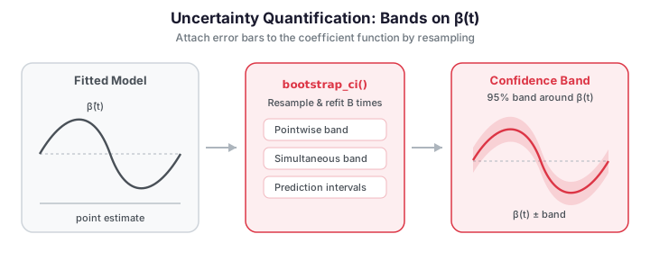
A point estimate of the coefficient function \(\hat\beta(t)\) or a single predicted response \(\hat y\) tells you what the model believes, but not how much to trust it. Uncertainty quantification attaches error bars: a confidence band around \(\beta(t)\) that shows where the predictor genuinely drives the response, and prediction intervals around \(\hat y\) that bracket where a new observation is likely to fall.

fdars supports two complementary routes. Bootstrapping (bootstrap_ci_fregre_lm) resamples the data to trace the sampling distribution of the whole coefficient function, producing both pointwise and simultaneous bands. Analytic prediction intervals (fdars.explain.prediction_intervals) propagate residual variance through the fitted model to bracket new responses. Neither requires distributional assumptions beyond the model itself — for distribution-free guarantees, see conformal prediction.

import numpy as np
from docs_fig import fig, render
from fdars.simulation import simulate
from fdars.regression import bootstrap_ci_fregre_lm

np.random.seed(0)
t = np.linspace(0, 1, 60)
X = np.asarray(simulate(n=40, argvals=t, n_basis=6, efun_type="fourier", seed=1))
beta_true = np.sin(2 * np.pi * t)
y = np.trapezoid(X * beta_true, t, axis=1) + 0.3 * np.random.randn(len(X))

ci = bootstrap_ci_fregre_lm(X, y, n_comp=4, n_boot=200, alpha=0.05, seed=1)
center = np.asarray(ci["center"])
lo, hi = np.asarray(ci["lower"]), np.asarray(ci["upper"])
slo, shi = np.asarray(ci["sim_lower"]), np.asarray(ci["sim_upper"])

f, ax = fig()
ax.fill_between(t, slo, shi, color="#3f51b5", alpha=0.12, label="95% simultaneous")
ax.fill_between(t, lo, hi, color="#3f51b5", alpha=0.28, label="95% pointwise")
ax.plot(t, center, color="#3f51b5", lw=2, label=r"$\hat\beta(t)$")
ax.axhline(0, color="#6c757d", lw=1, ls=":")
ax.set(title="Bootstrap confidence band for the coefficient function",
       xlabel="t", ylabel=r"$\beta(t)$")
ax.legend(fontsize=8)
print(render(f))

Where the band excludes zero, the predictor's contribution at that \(t\) is statistically distinguishable from none — a functional analogue of a significant coefficient.

Concepts

Bootstrap confidence bands. Refit the model on \(B\) resamples of the data to obtain \(\hat\beta^{(1)}(t),\dots,\hat\beta^{(B)}(t)\). At each \(t\), the \(\alpha/2\) and \(1-\alpha/2\) quantiles across the resamples give a pointwise band with \(1-\alpha\) coverage at every fixed \(t\). But a pointwise band under-covers the whole curve: the chance that \(\beta(t)\) falls inside the band at all \(t\) simultaneously is well below \(1-\alpha\). A simultaneous band widens the interval by a common factor so that the entire true curve lies inside with probability \(1-\alpha\) — the honest choice when you want to make statements about \(\beta\) as a function.

Prediction intervals. For a new curve \(x^*\), the predicted response \(\hat y^* = \hat\alpha + \int x^*(t)\hat\beta(t)\,dt\) carries two sources of error: uncertainty in the estimated model and the irreducible noise \(\varepsilon\). The prediction interval

\[ \hat y^* \pm t_{n-p,\,1-\alpha/2}\,\hat\sigma\sqrt{1 + z^{*\top}(Z^\top Z)^{-1}z^*} \]

accounts for both (the leading \(1\) under the root is the noise term), and is therefore wider than a confidence interval for the mean response.

Bootstrap bands — bootstrap_ci_fregre_lm

import numpy as np
from fdars.simulation import simulate
from fdars.regression import bootstrap_ci_fregre_lm

np.random.seed(0)
t = np.linspace(0, 1, 60)
X = np.asarray(simulate(n=40, argvals=t, n_basis=6, efun_type="fourier", seed=1))
beta_true = np.sin(2 * np.pi * t)
y = np.trapezoid(X * beta_true, t, axis=1) + 0.3 * np.random.randn(len(X))

ci = bootstrap_ci_fregre_lm(X, y, n_comp=4, n_boot=200, alpha=0.05, seed=1)
width = np.asarray(ci["upper"]) - np.asarray(ci["lower"])
print(f"mean pointwise band width: {width.mean():.3f}")
print(f"successful bootstrap fits: {int(ci['n_boot_success'])}")

Parameter	Type	Description
data	ndarray (n, m)	Functional predictors
response	ndarray (n,)	Scalar response
n_comp	int	Number of FPC components
n_boot	int	Bootstrap resamples (default 200)
alpha	float	Miscoverage level; \(1-\alpha\) coverage
seed	int	Random seed

Return key	Type	Description
center	ndarray (m,)	Point estimate \(\hat\beta(t)\)
lower, upper	ndarray (m,)	Pointwise \(1-\alpha\) band
sim_lower, sim_upper	ndarray (m,)	Simultaneous \(1-\alpha\) band
n_boot_success	float	Number of resamples that fit successfully

Prediction intervals — prediction_intervals

Given held-out curves, prediction_intervals returns a bracketed prediction for each, using the residual scale and design leverage of the new points.

import numpy as np
from fdars.explain import prediction_intervals

# fit on the first 30, predict-with-intervals on the last 10
pi = prediction_intervals(X[:30], y[:30], X[30:], ncomp=4, confidence_level=0.95)
covered = np.mean((y[30:] >= pi["lower"]) & (y[30:] <= pi["upper"]))
print(f"empirical coverage on held-out: {covered:.2f}")

Return key	Type	Description
predictions	ndarray (n_new,)	Point predictions \(\hat y^*\)
lower, upper	ndarray (n_new,)	Prediction interval bounds
prediction_se	ndarray (n_new,)	Standard error of each prediction
confidence_level	float	Nominal coverage
t_critical	float	\(t\) quantile used
residual_se	float	Residual scale \(\hat\sigma\)

Nearly every orange observed value falls inside its blue 95% interval, the visual signature of valid coverage on held-out curves. The intervals are roughly constant in width here because the simulated noise is homoscedastic; in real data the bars would widen for predictions made far from the training curves, flagging where the model is least sure.

Coverage and width

Two numbers summarize a prediction interval: does it cover the truth at the nominal rate, and how wide is it? Parametric intervals widen for high-leverage test points — curves whose FPC-score profile sits far from the training center — because the leverage term \(z^{*\top}(Z^\top Z)^{-1}z^*\) under the root grows. That variable width is the interval honestly reporting where the model is extrapolating.

import numpy as np
from docs_fig import fig, render
from fdars.simulation import simulate
from fdars.explain import prediction_intervals

np.random.seed(0)
t = np.linspace(0, 1, 60)
X = np.asarray(simulate(n=40, argvals=t, n_basis=6, efun_type="fourier", seed=1))
beta_true = np.sin(2 * np.pi * t)
y = np.trapezoid(X * beta_true, t, axis=1) + 0.3 * np.random.randn(len(X))

pi = prediction_intervals(X[:30], y[:30], X[30:], ncomp=4, confidence_level=0.95)
lo, hi = np.asarray(pi["lower"]), np.asarray(pi["upper"])
width = hi - lo
covered = float(np.mean((y[30:] >= lo) & (y[30:] <= hi)))

f, ax = fig()
ax.bar(np.arange(len(width)), width, color="#7b2d8e", alpha=0.75)
ax.set(title=f"Prediction-interval width (coverage = {covered*100:.0f}%, nominal 95%)",
       xlabel="held-out observation", ylabel="interval width")
print(render(f))

Empirical coverage lands near the 95% target and the widths vary point-to-point with leverage. Parametric intervals are exact only when the errors are Gaussian; the regression diagnostics Q-Q plot is the check that justifies them.

Validation — both intervals cover at their nominal rate

A single split is noisy, so we average over many independent draws. (1) The prediction intervals must cover held-out responses at ~the nominal \(1-\alpha\) rate. (2) The bootstrap simultaneous band must contain the entire true \(\beta(t)\) curve at ≥ its nominal rate (it is a conservative, whole-curve guarantee). Both assertions run and pass below.

import numpy as np
from fdars.simulation import simulate
from fdars.regression import bootstrap_ci_fregre_lm
from fdars.explain import prediction_intervals

t = np.linspace(0, 1, 60)
beta_true = np.sin(2 * np.pi * t)

# (1) Prediction-interval coverage on held-out data, averaged over 40 draws.
pi_cov = []
for rep in range(40):
    rng = np.random.default_rng(200 + rep)
    X = np.asarray(simulate(n=60, argvals=t, n_basis=6, efun_type="fourier", seed=rep))
    y = np.trapezoid(X * beta_true, t, axis=1) + 0.3 * rng.standard_normal(len(X))
    pi = prediction_intervals(X[:40], y[:40], X[40:], ncomp=4, confidence_level=0.90)
    lo, hi = np.asarray(pi["lower"]), np.asarray(pi["upper"])
    pi_cov.append(float(np.mean((y[40:] >= lo) & (y[40:] <= hi))))
mean_pi_cov = float(np.mean(pi_cov))

# (2) Bootstrap simultaneous band: does it contain the whole true beta(t)?
sim_hits = []
for rep in range(20):
    rng = np.random.default_rng(300 + rep)
    X = np.asarray(simulate(n=60, argvals=t, n_basis=6, efun_type="fourier", seed=rep))
    y = np.trapezoid(X * beta_true, t, axis=1) + 0.3 * rng.standard_normal(len(X))
    ci = bootstrap_ci_fregre_lm(X, y, n_comp=4, n_boot=200, alpha=0.05, seed=rep)
    slo, shi = np.asarray(ci["sim_lower"]), np.asarray(ci["sim_upper"])
    sim_hits.append(bool(np.all((beta_true >= slo) & (beta_true <= shi))))
sim_band_cov = float(np.mean(sim_hits))

print(f"prediction-interval coverage (nominal 0.90) = {mean_pi_cov:.3f}")
print(f"simultaneous-band beta(t) coverage (>=0.95) = {sim_band_cov:.3f}")

assert abs(mean_pi_cov - 0.90) < 0.05, mean_pi_cov
assert sim_band_cov >= 0.95, sim_band_cov
print("validation OK: PI coverage ~= nominal, and the simultaneous band covers beta(t)")

prediction-interval coverage (nominal 0.90) = 0.912 simultaneous-band beta(t) coverage (>=0.95) = 1.000 validation OK: PI coverage ~= nominal, and the simultaneous band covers beta(t)

The prediction-interval coverage lands within a few points of the 90% target, and the simultaneous band brackets the entire true \(\beta(t)\) in every replicate — the honest, conservative behaviour a whole-curve guarantee should show.

Parametric vs. distribution-free width

When the Gaussian assumption is shaky, conformal prediction trades the parametric formula for a calibration step that guarantees coverage regardless of the error distribution. The split-conformal variant produces a constant-width band (one calibration quantile applied to every test point), which is the visible signature separating it from the leverage-dependent parametric width.

import numpy as np
from docs_fig import fig, render
from fdars.simulation import simulate
from fdars.explain import prediction_intervals
from fdars.conformal import conformal_fregre_lm

np.random.seed(0)
t = np.linspace(0, 1, 60)
# Larger sample so the split-conformal calibration set is big enough for a
# finite 90% quantile.
X = np.asarray(simulate(n=80, argvals=t, n_basis=6, efun_type="fourier", seed=1))
beta_true = np.sin(2 * np.pi * t)
y = np.trapezoid(X * beta_true, t, axis=1) + 0.3 * np.random.randn(len(X))

# Both at 90% nominal, fit on the first 60 and predict the last 20.
pi = prediction_intervals(X[:60], y[:60], X[60:], ncomp=4, confidence_level=0.90)
param_w = np.asarray(pi["upper"]) - np.asarray(pi["lower"])
cf = conformal_fregre_lm(X[:60], y[:60], X[60:], ncomp=4, cal_fraction=0.25,
                         alpha=0.10, seed=42)
conf_w = np.asarray(cf["upper"]) - np.asarray(cf["lower"])

f, ax = fig()
ax.boxplot([param_w, conf_w], tick_labels=["parametric", "conformal"])
ax.set(title="Interval width: parametric vs. split conformal (90% nominal)",
       ylabel="interval width")
print(render(f))

The conformal widths collapse to a single value; the parametric widths spread out with leverage. Which you prefer depends on whether you trust the Gaussian model (parametric, leverage-adaptive) or want a finite-sample guarantee (conformal, assumption-free). Here the conformal band is actually the tighter of the two on average — the parametric formula inflates its width to hedge against the Gaussian tails — so the distribution-free option costs nothing in width on this data.

Model assessment: leave-one-out CV — loo_cv_press

A confidence band tells you about the coefficient; leave-one-out cross-validation tells you about the model as a whole — can it predict a point it has never seen? For the linear FPC model there is no need to refit \(n\) times: the hat matrix gives every leave-one-out residual in closed form,

\[ e_i^{(-i)} = \frac{e_i}{1 - h_{ii}}, \]

which inflates each in-sample residual by \(1/(1-h_{ii})\) — a factor that grows with leverage. Summing their squares gives the PRESS statistic and an out-of-sample \(R^2\):

\[ \text{PRESS} = \sum_i \big(e_i^{(-i)}\big)^2, \qquad R^2_{\text{LOO}} = 1 - \frac{\text{PRESS}}{\text{TSS}}. \]

from fdars.explain import loo_cv_press

loo = loo_cv_press(X, y, ncomp=4)
print(f"PRESS:   {loo['press']:.3f}")
print(f"LOO R²:  {loo['loo_r_squared']:.3f}")

The gap between \(R^2_{\text{LOO}}\) and the in-sample \(R^2\) measures how optimistic the training fit is. High-leverage points drive that gap: their LOO residuals inflate most.

import numpy as np
from docs_fig import fig, render
from fdars.simulation import simulate
from fdars.explain import loo_cv_press

np.random.seed(0)
t = np.linspace(0, 1, 60)
X = np.asarray(simulate(n=40, argvals=t, n_basis=6, efun_type="fourier", seed=1))
beta_true = np.sin(2 * np.pi * t)
y = np.trapezoid(X * beta_true, t, axis=1) + 0.3 * np.random.randn(len(X))

loo = loo_cv_press(X, y, ncomp=4)
loo_res = np.asarray(loo["loo_residuals"])
lev = np.asarray(loo["leverage"])
# in-sample residual = loo_residual * (1 - leverage)
in_res = loo_res * (1 - lev)

f, ax = fig()
lim = [min(in_res.min(), loo_res.min()), max(in_res.max(), loo_res.max())]
ax.plot(lim, lim, color="#6c757d", ls="--", lw=1)
ax.scatter(in_res, loo_res, color="#7b2d8e", s=36, alpha=0.75)
ax.set(title=f"In-sample vs. LOO residuals (LOO R² = {loo['loo_r_squared']:.3f})",
       xlabel="in-sample residual", ylabel="LOO residual")
print(render(f))

Points drift off the diagonal exactly where leverage is high — those are the observations the model leans on to fit itself, and the ones a train/test split would penalize.

Return key	Type	Description
loo_residuals	ndarray (n,)	Leave-one-out residuals \(e_i^{(-i)}\)
press	float	Predicted residual sum of squares
loo_r_squared	float	Out-of-sample \(R^2\)
leverage	ndarray (n,)	Hat-matrix diagonal \(h_{ii}\)
tss	float	Total sum of squares of the response

Pointwise or simultaneous?

Use the pointwise band to ask "is \(\beta\) nonzero here?" at a pre-specified \(t\). Use the simultaneous band whenever you scan the whole curve for regions of significance — otherwise multiple-comparison inflation makes spurious excursions look real.

Bootstrap vs. conformal

Bootstrap bands and analytic intervals are only as valid as the model and its noise assumptions. Conformal prediction instead wraps any fitted model in a calibration step that delivers finite-sample, distribution-free coverage — at the cost of holding out calibration data. The two are complementary: bootstrap for interpreting \(\beta(t)\), conformal for guaranteed predictive coverage.

Related pages

• Conformal prediction — distribution-free predictive intervals.
• Regression diagnostics — check for influential points before trusting a band.
• Scalar-on-function regression — the underlying model being quantified.

References

• Efron, B., & Tibshirani, R. J. (1993). An Introduction to the Bootstrap. Chapman & Hall.
• Ramsay, J. O., & Silverman, B. W. (2005). Functional Data Analysis (2nd ed.). Springer.
• Cardot, H., Ferraty, F., & Sarda, P. (2003). Spline estimators for the functional linear model. Statistica Sinica, 13(3), 571–591.
• Horváth, L., & Kokoszka, P. (2012). Inference for Functional Data with Applications. Springer.