Cross-Validation: Honest Model Comparison with OOF Predictions

Dataset: Tecator — near-infrared absorbance spectra (100 channels, 850–1050 nm) of 240 meat samples, each with a lab-measured fat content.

A model that has seen a point can predict it well; that tells us almost nothing about a new sample. When we pick a functional regression model — how many components, which method — the temptation is to fit on all the data and read off the resulting \(R^2\). That number is optimistic: it rewards memorisation. The honest question is how well would this predict a meat sample we have not measured yet?

Cross-validation answers it by rotating every observation through a held-out fold, so that each sample is predicted by a model that never saw it. Collecting those held-out predictions gives an out-of-fold (OOF) prediction for every sample, from which a single honest error estimate falls out. This page uses the Tecator spectra to predict fat and compares three functional regressions on that honest footing.

Let \(\kappa(i)\in\{1,\dots,K\}\) be the fold holding sample \(i\), and let \(\hat f^{(-\kappa(i))}\) denote the model trained on every fold except \(\kappa(i)\). The out-of-fold prediction for sample \(i\) is that held-out model evaluated on curve \(x_i\), and the honest error is their mean square:

\[ \hat y_i^{\text{OOF}} = \hat f^{(-\kappa(i))}(x_i), \qquad \text{MSE}_{\text{OOF}} = \frac{1}{n}\sum_{i=1}^{n} \bigl(y_i - \hat y_i^{\text{OOF}}\bigr)^2 . \]

The corresponding honest coefficient of determination compares that error to the variance of the response, so \(R^2_{\text{OOF}} = 1\) is perfect prediction and \(R^2_{\text{OOF}} = 0\) matches the constant mean:

\[ R^2_{\text{OOF}} = 1 - \frac{\sum_{i}(y_i - \hat y_i^{\text{OOF}})^2} {\sum_{i}(y_i - \bar y)^2} . \]

The optimism of the in-sample fit

We start with the FPC linear model (fregre_lm): project each spectrum onto its leading functional principal components, then regress fat on those scores. The knob is the number of components. Adding components can only improve the fit to the data the model was trained on — but past a point those extra components fit noise, not signal. Plotting the in-sample \(R^2\) against the honest OOF \(R^2\) makes the gap visible.

import numpy as np
from docs_fig import fig, render
from docs_data import load_tecator
from fdars.fdata import deriv_1d
from fdars.regression import fregre_lm, predict_fregre_lm

wl, X, meta = load_tecator()
fat = meta["fat"].to_numpy()
D2 = np.asarray(deriv_1d(X, wl, nderiv=2))       # baseline-corrected spectra
n = len(fat)

rng = np.random.default_rng(0)
folds = rng.integers(0, 5, n)                     # 5-fold assignment
def r2(y, p): return 1 - np.sum((y - p) ** 2) / np.sum((y - y.mean()) ** 2)

ncomps = [2, 5, 10, 15, 20, 25, 30]
r2_in, r2_oof = [], []
for nc in ncomps:
    ins = np.asarray(fregre_lm(D2, fat, n_comp=nc)["fitted_values"])
    oof = np.empty(n)
    for k in range(5):                            # rotate held-out fold
        te = folds == k
        oof[te] = np.asarray(
            predict_fregre_lm(D2[~te], fat[~te], D2[te], n_comp=nc))
    r2_in.append(r2(fat, ins))
    r2_oof.append(r2(fat, oof))

f, ax = fig()
ax.plot(ncomps, r2_in, "o-", color="#dc3545", lw=2, label="in-sample $R^2$")
ax.plot(ncomps, r2_oof, "o-", color="#3f51b5", lw=2, label="out-of-fold $R^2$")
ax.fill_between(ncomps, r2_oof, r2_in, color="#dc3545", alpha=0.10)
ax.set(title="In-sample $R^2$ keeps rising; honest $R^2$ does not",
       xlabel="number of FPC components", ylabel="$R^2$")
ax.legend(loc="lower right")
print(render(f))

The red curve climbs monotonically — more components always fit the training data better. The blue OOF curve peaks and then declines: beyond roughly 20 components the model is memorising noise, and its honest accuracy gets worse even as the in-sample number keeps improving. The shaded gap between the two is the optimism you pay for by trusting the in-sample fit.

Validation — optimism is non-negative, and CV picks a sane \(k\)

The whole page rests on one inequality that must hold by construction: a model's out-of-fold error can never be smaller than its in-sample error for the same complexity — the gap is the optimism, \(\text{opt} = \text{MSE}_{\text{OOF}} - \text{MSE}_{\text{in}} \ge 0\). We assert \(\text{MSE}_{\text{OOF}} \ge \text{MSE}_{\text{in}}\) at a fixed component count. We also assert fregre_cv returns an optimal_k inside the searched range \([1, 12]\) (not a degenerate 0 or an out-of-range index).

import numpy as np
from docs_data import load_tecator
from fdars.fdata import deriv_1d
from fdars.regression import fregre_lm, predict_fregre_lm, fregre_cv

wl, X, meta = load_tecator()
fat = meta["fat"].to_numpy()
D2 = np.asarray(deriv_1d(X, wl, nderiv=2))
n = len(fat)
rng = np.random.default_rng(0)
folds = rng.integers(0, 5, n)
mse = lambda y, p: float(np.mean((y - p) ** 2))

# (1) OOF error >= in-sample error at fixed complexity (the optimism gap)
nc = 20
ins = np.asarray(fregre_lm(D2, fat, n_comp=nc)["fitted_values"])
oof = np.empty(n)
for k in range(5):
    te = folds == k
    oof[te] = np.asarray(predict_fregre_lm(D2[~te], fat[~te], D2[te], n_comp=nc))
e_in, e_oof = mse(fat, ins), mse(fat, oof)
assert e_oof >= e_in, (e_oof, e_in)

# (2) fregre_cv selects a component count inside the searched range
kbest = int(fregre_cv(D2, fat, k_min=1, k_max=12, n_folds=5)["optimal_k"])
assert 1 <= kbest <= 12, kbest
print(f"in-sample MSE {e_in:.3f}  <=  OOF MSE {e_oof:.3f}  "
      f"(optimism {e_oof - e_in:.3f})")
print(f"fregre_cv optimal_k = {kbest}  (in [1, 12])")

in-sample MSE 4.548 <= OOF MSE 5.979 (optimism 1.431) fregre_cv optimal_k = 12 (in [1, 12])

Both hold: the honest error exceeds the in-sample error by the optimism gap, and the cross-validated component count is a sane value inside the search grid — the machinery is measuring generalisation, not memorisation.

Choosing the number of components

Rather than eyeball the elbow, fregre_cv runs the fold rotation internally and reports the cross-validated error for each component count, together with the OOF prediction for every sample. It returns the optimal \(k\), the per-\(k\) CV errors, and the OOF predictions and fold assignments.

import numpy as np
from docs_fig import fig, render
from docs_data import load_tecator
from fdars.fdata import deriv_1d
from fdars.regression import fregre_cv

wl, X, meta = load_tecator()
fat = meta["fat"].to_numpy()
D2 = np.asarray(deriv_1d(X, wl, nderiv=2))

cv = fregre_cv(D2, fat, k_min=1, k_max=25, n_folds=5)
kk = np.asarray(cv["k_values"])
err = np.asarray(cv["cv_errors"])
kbest = int(cv["optimal_k"])

f, ax = fig()
ax.plot(kk, err, "o-", color="#3f51b5", lw=2)
ax.axvline(kbest, color="#e8710a", ls="--", lw=1.5,
           label=f"optimal $k$ = {kbest}")
ax.scatter([kbest], [cv["min_cv_error"]], color="#e8710a", s=70, zorder=5)
ax.set(title="Cross-validated error vs number of components",
       xlabel="number of FPC components", ylabel="CV mean squared error")
ax.legend()
print(render(f))

The CV error drops steeply through the first dozen or so components, then bends into a long, shallow decline before bottoming out and ticking back up — so the minimum is a genuine interior optimum, not an artefact of stopping the search too early. fregre_cv marks the component count that minimises the curve. The visual elbow — where each extra component stops buying much — sits around a dozen components; past it the curve keeps inching down to its flat minimum, so anything from the elbow onward is a defensible choice, trading a little honest accuracy for a simpler model.

fregre_cv returns the OOF predictions for free

Besides optimal_k, min_cv_error, k_values and cv_errors, the returned dict carries oof_predictions (one honest prediction per sample) and fold_assignments — exactly what we need to plot predicted-vs-actual below without re-running the folds ourselves.

OOF predicted vs. actual, colored by fold

The single most informative cross-validation plot: every sample's honest prediction against its measured fat, colored by the fold that produced it. If a particular fold were systematically off, its color would sit off the diagonal.

import numpy as np
import matplotlib.cm as cm
from docs_fig import fig, render
from docs_data import load_tecator
from fdars.fdata import deriv_1d
from fdars.regression import fregre_cv

wl, X, meta = load_tecator()
fat = meta["fat"].to_numpy()
D2 = np.asarray(deriv_1d(X, wl, nderiv=2))

cv = fregre_cv(D2, fat, k_min=1, k_max=12, n_folds=5)
oof = np.asarray(cv["oof_predictions"])
fold = np.asarray(cv["fold_assignments"])
r2_oof = 1 - np.sum((fat - oof) ** 2) / np.sum((fat - fat.mean()) ** 2)

f, ax = fig(figsize=(5.2, 5.0))
lim = [fat.min() - 2, fat.max() + 2]
ax.plot(lim, lim, color="#6c757d", ls=":", lw=1)
for k in np.unique(fold):
    m = fold == k
    ax.scatter(fat[m], oof[m], s=26, alpha=0.85, edgecolor="white",
               color=cm.tab10(k / 10), label=f"fold {k}")
ax.set(title=f"Out-of-fold predictions (honest $R^2$ = {r2_oof:.3f})",
       xlabel="measured fat (%)", ylabel="OOF predicted fat (%)",
       xlim=lim, ylim=lim)
ax.legend(title="held-out fold", fontsize=8)
print(render(f))

The folds intermix along the diagonal — no single fold is an outlier, so the honest \(R^2\) is a trustworthy summary rather than an artefact of one lucky split.

Per-fold stability

A single OOF \(R^2\) hides whether the model is equally good on every split. The most direct stability check is a boxplot of the residuals within each fold: if one fold's box sits off zero or is far wider than the others, the summary error is being propped up (or dragged down) by a lucky partition rather than reflecting genuine generalisation.

import numpy as np
from docs_fig import fig, render
from docs_data import load_tecator
from fdars.fdata import deriv_1d
from fdars.regression import fregre_cv

wl, X, meta = load_tecator()
fat = meta["fat"].to_numpy()
D2 = np.asarray(deriv_1d(X, wl, nderiv=2))

cv = fregre_cv(D2, fat, k_min=1, k_max=12, n_folds=5)
oof = np.asarray(cv["oof_predictions"])
fold = np.asarray(cv["fold_assignments"])
resid = fat - oof
by_fold = [resid[fold == k] for k in np.unique(fold)]

f, ax = fig()
ax.axhline(0, color="#dc3545", ls="--", lw=1)
bp = ax.boxplot(by_fold, patch_artist=True,
                tick_labels=[f"fold {k}" for k in np.unique(fold)])
for box in bp["boxes"]:
    box.set(facecolor="#cfe0ff", alpha=0.8)
ax.set(title="Out-of-fold residuals by fold",
       xlabel="held-out fold", ylabel="residual (measured − OOF)")
print(render(f))

The boxes straddle zero with comparable spreads — no fold is systematically biased, so the cross-validated error is a stable estimate, not the product of one fortunate split.

Stratified folds keep each split representative

Random fold assignment can, by chance, load the high-fat samples into a couple of folds and starve the others — a real risk here because the Tecator fat distribution is right-skewed. Stratified folds instead spread the response evenly across folds, so every fold sees a similar range of fat. fdars does not expose a fold builder, so we stratify transparently: sort by fat and deal samples round-robin into folds.

import numpy as np
from docs_fig import fig, render
from docs_data import load_tecator

wl, X, meta = load_tecator()
fat = meta["fat"].to_numpy()
n = len(fat)

def stratified_folds(y, k, seed=1):
    folds = np.empty(len(y), dtype=int)
    for i, idx in enumerate(np.argsort(y)):   # round-robin along sorted y
        folds[idx] = i % k
    return folds

fs = stratified_folds(fat, 5)
fr = np.random.default_rng(1).integers(0, 5, n)

f, (aL, aR) = fig(ncols=2, figsize=(9.4, 3.7))
for ax, folds, ttl in [(aL, fs, "Stratified"), (aR, fr, "Random")]:
    groups = [fat[folds == k] for k in range(5)]
    ax.boxplot(groups, patch_artist=True,
               tick_labels=[str(k) for k in range(5)])
    spread = np.ptp([g.mean() for g in groups])
    ax.set(title=f"{ttl}  (fold-mean spread {spread:.1f}%)",
           xlabel="fold", ylabel="fat (%)")
print(render(f))

The random folds' means scatter over several percent of fat; the stratified folds are nearly identical. When the response is skewed, stratifying removes a source of noise from the CV estimate — each fold is a fair miniature of the whole dataset.

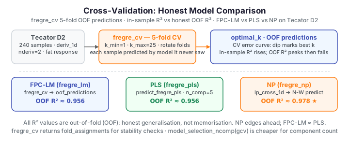
Comparing three models honestly

FPC-LM is only one option. Functional PLS (fregre_pls) chooses components that covary with the response instead of maximising spectral variance; nonparametric regression (fregre_np) abandons a coefficient curve entirely and predicts each sample from a kernel-weighted average of its neighbours in curve space. The only fair comparison is OOF against OOF. We rotate the same five folds through all three.

fregre_cv already gives us the FPC-LM OOF predictions. PLS has a matching predict_fregre_pls, so we run its folds directly. fregre_np has no separate predict binding, so we form its prediction transparently: fit on the training distance matrix to get its bandwidth h_func, then apply the Nadaraya–Watson kernel average using the cross distances between held-out and training spectra (fdars.metric.lp_cross_1d).

import numpy as np
from docs_fig import fig, render
from docs_data import load_tecator
from fdars.fdata import deriv_1d
from fdars.metric import lp_self_1d, lp_cross_1d
from fdars.regression import fregre_cv, predict_fregre_pls, fregre_np

wl, X, meta = load_tecator()
fat = meta["fat"].to_numpy()
D2 = np.asarray(deriv_1d(X, wl, nderiv=2))
n = len(fat)
rng = np.random.default_rng(0)
folds = rng.integers(0, 5, n)
def r2(y, p): return 1 - np.sum((y - p) ** 2) / np.sum((y - y.mean()) ** 2)

# FPC-LM: built-in OOF
oof_lm = np.asarray(fregre_cv(D2, fat, k_min=1, k_max=12, n_folds=5)["oof_predictions"])

# PLS: manual folds (n_comp kept modest — see warning)
oof_pls = np.empty(n)
for k in range(5):
    te = folds == k
    oof_pls[te] = np.asarray(
        predict_fregre_pls(D2[~te], wl, fat[~te], D2[te], n_comp=5))

# NP: manual folds, Nadaraya–Watson via cross distances
oof_np = np.empty(n)
for k in range(5):
    te = folds == k; tr = ~te
    h = fregre_np(np.asarray(lp_self_1d(D2[tr], wl, 2.0)), fat[tr], 0.0)["h_func"]
    Dc = np.asarray(lp_cross_1d(D2[te], D2[tr], wl, 2.0))    # (n_te, n_tr)
    W = np.exp(-0.5 * (Dc / h) ** 2)
    oof_np[te] = (W @ fat[tr]) / W.sum(1)

names = ["FPC-LM", "PLS", "NP"]
scores = [r2(fat, oof_lm), r2(fat, oof_pls), r2(fat, oof_np)]

f, ax = fig()
bars = ax.bar(names, scores, color=["#3f51b5", "#198754", "#e8710a"], width=0.6)
for b, s in zip(bars, scores):
    ax.text(b.get_x() + b.get_width() / 2, s + 0.002, f"{s:.3f}",
            ha="center", va="bottom", fontsize=10)
ax.set(title="Honest (out-of-fold) $R^2$ by model",
       ylabel="OOF $R^2$", ylim=(0.90, 1.0))
print(render(f))

On these second-derivative spectra all three models clear an OOF \(R^2\) of 0.95. The nonparametric neighbour model edges clearly ahead (~0.978), while PLS and the FPC linear model are effectively tied (~0.956 apiece) — the linear methods extract the same predictive signal here, and neither has an edge over the other. Because every number is out-of-fold, this ranking reflects predictive ability, not fitting capacity.

PLS component count on collinear spectra

fregre_pls factorises a covariance matrix with a Cholesky decomposition. On the Tecator spectra — whose 100 channels are highly collinear — that matrix goes singular once n_comp reaches about 7, raising Cholesky factorization failed: matrix is singular or near-singular. We keep n_comp = 5 here. If you need more components, work on the second-derivative spectra (as we do) and/or select the count by cross-validation rather than pushing it higher.

Parameters

Function	Key parameters	Description
fregre_cv(data, response, k_min, k_max, n_folds)	k_min, k_max, n_folds	Range of FPC components to test; number of CV folds
fregre_lm(data, response, n_comp)	n_comp	Number of FPC components in the linear model
predict_fregre_lm(data_fit, response, new_data, n_comp)	new_data	Spectra to predict from a refit model
fregre_pls(data, argvals, response, n_comp)	n_comp	Number of PLS components
predict_fregre_pls(data, argvals, response, new_data, n_comp)	new_data	Spectra to predict
fregre_np(dist_matrix, response, h)	h	Kernel bandwidth (0 = auto, returned as h_func)

The dict from fregre_cv contains optimal_k, min_cv_error, k_values, cv_errors, oof_predictions, fold_assignments, and fold_errors.

model_selection_ncomp for a criterion-based choice

If you would rather select the component count by an information criterion than by fold rotation, model_selection_ncomp(data, response, max_comp, criterion="gcv") returns best_ncomp and a criteria matrix of (ncomp, aic, bic, gcv) rows — a cheaper alternative to full CV when you only need to pick \(k\).

See also

• Predicting fat from NIR spectra — the held-out PLS fit and coefficient curve on this same dataset.
• Explainability: recovering predictive regions — once a model is chosen, which wavelengths drive its predictions.
• Scalar-on-function regression for the functional linear model in general.

References

• Stone, M. (1974). Cross-validatory choice and assessment of statistical predictions. JRSS B 36(2):111-147.
• Ramsay, J.O., Silverman, B.W. (2005). Functional Data Analysis, 2nd ed. Springer.
• Febrero-Bande, M., Oviedo de la Fuente, M. (2012). Statistical computing in functional data analysis: fda.usc. JSS 51(4):1-28.
• Borggaard, C., Thodberg, H.H. (1992). Optimal minimal neural interpretation of spectra. Analytical Chemistry 64(5):545-551.