Functional Generalized Linear Model
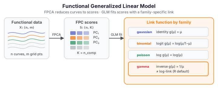
Functional GLM extends scalar-on-function regression to exponential-family responses. Instead of a Gaussian error term, the response may be binary (binomial), a count (Poisson), a positive continuous value (gamma), or unrestricted Gaussian. fdars.regression.functional_glm first projects each observed curve onto a small number of functional principal components (FPCA), then fits a standard GLM on the resulting scores — one scalar score per FPC per subject. The coefficient function \(\hat\beta(t)\) is reconstructed back to the original domain by recombining the FPC loadings.
When to use
Use functional_glm when your response variable is not Gaussian — binary outcomes, counts, or strictly positive continuous values — and your predictors are functional (curves). For a Gaussian response with a functional predictor, functional_glm with family="gaussian" produces the same fit as the linear scalar-on-function model, but the dedicated fregre_lm in fdars.regression is simpler.
| Situation | Recommended | fdars function |
|---|---|---|
| Binary response (0/1), pure classification task | Specialized logistic | fdars.regression.functional_logistic |
| Binary response, need β(t) and GLM diagnostics | Functional GLM | functional_glm(..., family="binomial") |
| Count response (non-negative integers) | Functional GLM | functional_glm(..., family="poisson") |
| Positive continuous response | Functional GLM | functional_glm(..., family="gamma") |
| Gaussian/unrestricted continuous response | Linear SoF | fdars.regression.fregre_lm |
Quick rule: Start with functional_glm when the response distribution dictates a non-identity link. For binary classification where predicted classes matter more than the coefficient function, prefer functional_logistic — it returns predicted classes directly and supports bootstrap_ci_functional_logistic. For Gaussian responses, use the simpler scalar-on-function linear model.
When functional_logistic is preferred over binomial GLM
fdars.regression.functional_logistic is a dedicated binary classifier that predates
functional_glm. It returns probabilities and predicted_classes directly, and it
supports bootstrap_ci_functional_logistic for confidence intervals on the coefficient
function. If your goal is to predict class labels rather than interpret β(t), use
functional_logistic from fdars.regression.
Theory
Let \(X_1(t), \dots, X_n(t)\) be \(n\) functional observations on grid \(t_1, \dots, t_m\), and let \(y_1, \dots, y_n\) be scalar responses from a specified exponential-family distribution. The model proceeds in two stages:
Stage 1 — FPCA projection. Decompose the functional data into n_comp leading functional principal components \(\phi_1(t), \dots, \phi_K(t)\) and form the score matrix \(S \in \mathbb{R}^{n \times K}\) where \(s_{ik} = \int X_i(t)\,\phi_k(t)\,dt\). Each curve is now represented by \(K\) scalar scores.
Stage 2 — GLM in score space. Fit a GLM on the scores:
where \(g(\cdot)\) is the link function for the chosen family and \(\gamma \in \mathbb{R}^K\) are scalar coefficients. The coefficient function on the original domain is
The GLM is fit by iteratively reweighted least squares (IRLS) with a maximum of max_iter iterations and convergence tolerance tol on the deviance change.
Link functions by family
| Family | Link | \(g(\mu)\) | Domain constraint | Notes |
|---|---|---|---|---|
"gaussian" |
identity | \(\mu\) | \(y \in \mathbb{R}\) | Reduces to ordinary functional linear model |
"binomial" |
logit | \(\log(\mu / (1-\mu))\) | \(y \in \{0, 1\}\) | Binary response |
"poisson" |
log | \(\log(\mu)\) | \(y \geq 0\) | Count response |
"gamma" |
inverse (canonical) | \(1/\mu\) | \(y > 0\) | Positive continuous; NOT log-link |
Gamma family uses the inverse canonical link, not log
fdars.regression.functional_glm with family="gamma" uses the inverse canonical link \(g(\mu) = 1/\mu\), not the log-link that R's glm(..., family=Gamma) defaults to. Results will differ from R if you assume a log-link. If you need a log-link for a Gamma response, transform the response before calling functional_glm with family="gaussian", or interpret the inverse-link coefficients appropriately.
AIC is not comparable to R glm() AIC
The AIC returned by functional_glm is computed from the score-space GLM log-likelihood, which treats the FPC scores as fixed predictors. This is not the same quantity as R's glm() AIC, which is based on the full-data likelihood. The AIC value here is useful for comparing models with different n_comp or family choices within fdars, but should not be compared numerically to AIC from R or other software.
Parameters
| Parameter | Type | Default | Description |
|---|---|---|---|
data |
ndarray (n, m) |
— | Functional data matrix; rows are observations |
response |
ndarray (n,) |
— | Scalar response vector |
family |
str |
"gaussian" |
Exponential family: "gaussian", "binomial", "poisson", "gamma" |
n_comp |
int |
3 |
Number of FPC components for the FPCA projection |
scalar_covariates |
ndarray (n, q) or None |
None |
Additional scalar predictors to include in the GLM alongside the FPC scores |
max_iter |
int |
25 |
Maximum IRLS iterations |
tol |
float |
1e-6 |
Convergence tolerance on deviance change |
Returns a dict with 15 keys:
| Key | Shape / Type | Description |
|---|---|---|
"intercept" |
float |
GLM intercept on the link scale |
"beta_t" |
(m,) |
Functional coefficient \(\hat\beta(t)\) on the original domain |
"beta_se" |
(m,) |
Pointwise standard errors of \(\hat\beta(t)\) |
"gamma" |
(K,) |
Score-space GLM coefficients (\(K\) = actual n_comp used) |
"fitted_values" |
(n,) |
Fitted responses on the response scale (inverse-linked) |
"linear_predictors" |
(n,) |
Linear predictors \(\hat\eta_i = \alpha + S_i^\top \hat\gamma\) |
"ncomp" |
int |
Actual number of FPC components used |
"coefficients" |
(K+1,) |
Full coefficient vector (intercept + score coefficients) |
"std_errors" |
(K+1,) |
Standard errors of coefficients |
"log_likelihood" |
float |
Log-likelihood of the fitted score-space GLM |
"deviance" |
float |
Residual deviance |
"iterations" |
int |
Number of IRLS iterations taken |
"aic" |
float |
AIC from the score-space GLM (not comparable to R glm AIC — see note above) |
"bic" |
float |
BIC from the score-space GLM |
"family" |
str |
Family string echoed back |
1. Binomial and Poisson examples
The code below fits the GLM for two families on synthetic data and plots the estimated coefficient functions. Each family uses a distinct link function and response domain.
import numpy as np
from docs_fig import fig, render
import fdars.regression as reg

rng = np.random.default_rng(1)
n, m = 30, 60
t = np.linspace(0, 1, m)
X = np.array([np.sin(2 * np.pi * t * (1 + 0.3 * rng.normal())) + rng.normal(0, 0.1, m)
              for _ in range(n)])

# --- Family 1: Binomial (binary response) ---
logit_true = X @ np.sin(2 * np.pi * t) / m
prob_true = 1 / (1 + np.exp(-3 * logit_true))
y_bin = rng.binomial(1, prob_true).astype(float)

res_bin = reg.functional_glm(X, y_bin, family="binomial", n_comp=3)
beta_bin = np.asarray(res_bin["beta_t"])

# --- Family 2: Poisson (count response, y >= 0) ---
# True log-rate is a linear functional of X; exp() ensures y >= 0.
log_rate_true = X @ np.cos(2 * np.pi * t) / m
y_poi = rng.poisson(np.exp(1.5 * log_rate_true)).astype(float)

res_poi = reg.functional_glm(X, y_poi, family="poisson", n_comp=3)
beta_poi = np.asarray(res_poi["beta_t"])

f, (a0, a1) = fig(1, 2, figsize=(12.0, 3.8))

a0.plot(t, beta_bin, color="#3f51b5", lw=2.2)
a0.set(title="Functional GLM (binomial) — β(t)",
       xlabel="t", ylabel="β(t)")

a1.plot(t, beta_poi, color="#e8710a", lw=2.2)
a1.set(title="Functional GLM (poisson) — β(t)",
       xlabel="t", ylabel="β(t)")

print(render(f))
print(f"binomial  deviance={res_bin['deviance']:.3f}  aic={res_bin['aic']:.3f}  "
      f"family={res_bin['family']}")
print(f"poisson   deviance={res_poi['deviance']:.3f}  aic={res_poi['aic']:.3f}  "
      f"family={res_poi['family']}")
print("FDARS_FENCE_OK")
2. Gaussian family — reduces to the linear scalar-on-function model
With family="gaussian" and the identity link, the functional GLM is algebraically equivalent to the linear scalar-on-function model (fregre_lm). This fence verifies that claim by comparing fitted values from both estimators on the same data.
import numpy as np
from fdars.regression import functional_glm, fregre_lm

rng = np.random.default_rng(42)
n, m = 25, 40
t = np.linspace(0, 1, m)

# Build functional data from 3 explicit FPC scores for good conditioning.
scores = rng.standard_normal((n, 3))
phi = np.array([np.sin((k + 1) * np.pi * t) for k in range(3)])
X = scores @ phi + 0.05 * rng.standard_normal((n, m))
y = X @ phi[0] / m + 0.2 * rng.standard_normal(n)

glm_g = functional_glm(X, y, family="gaussian", n_comp=3)
lm    = fregre_lm(X, y, n_comp=3)

corr = np.corrcoef(np.asarray(glm_g["fitted_values"]),
                   np.asarray(lm["fitted_values"]))[0, 1]
print(f"Correlation of fitted values (GLM gaussian vs fregre_lm): {corr:.6f}")
print(f"GLM  deviance={glm_g['deviance']:.4f}  aic={glm_g['aic']:.4f}")
print(f"fregre_lm r_squared={lm['r_squared']:.4f}")
print("FDARS_FENCE_OK")
Correlation of fitted values (GLM gaussian vs fregre_lm): 1.000000 GLM deviance=0.8910 aic=9.7820 fregre_lm r_squared=0.8201 FDARS_FENCE_OK
The correlation between fitted values is essentially 1.0 — confirming that the Gaussian functional GLM and the linear scalar-on-function model are equivalent estimators for Gaussian responses.
3. Choosing n_comp — parameter selection
n_comp controls how many FPCA components are retained before fitting the GLM. Too few components miss signal; too many add noise. Use model_selection_ncomp from fdars.scalar_on_function to select n_comp by GCV (generalized cross-validation), AIC, or BIC before fitting the GLM.
import numpy as np
from fdars.scalar_on_function import model_selection_ncomp
from fdars.regression import functional_glm

rng = np.random.default_rng(42)
n, m = 25, 40
t = np.linspace(0, 1, m)

scores = rng.standard_normal((n, 3))
phi = np.array([np.sin((k + 1) * np.pi * t) for k in range(3)])
X = scores @ phi + 0.05 * rng.standard_normal((n, m))
y = X @ phi[0] / m + 0.2 * rng.standard_normal(n)

# Select n_comp via GCV on the linear (Gaussian) sub-problem first.
sel = model_selection_ncomp(X, y, max_comp=6, criterion="gcv")
best = sel["best_ncomp"]

print(f"Best n_comp (GCV): {best}")
print("  n_comp | AIC      | BIC      | GCV")
for ncomp, aic, bic, gcv in sel["criteria"]:
    print(f"  {ncomp:6d} | {aic:8.2f} | {bic:8.2f} | {gcv:.5f}")

# Fit the GLM with the selected n_comp.
res = functional_glm(X, y, family="gaussian", n_comp=best)
print(f"\nGLM (gaussian, n_comp={best}): deviance={res['deviance']:.4f}  "
      f"aic={res['aic']:.4f}  iterations={res['iterations']}")
print("FDARS_FENCE_OK")
Best n_comp (GCV): 3 n_comp | AIC | BIC | GCV 1 | -51.36 | -48.92 | 0.12607 2 | -75.00 | -71.34 | 0.04997 3 | -75.36 | -70.48 | 0.04778 4 | -73.37 | -67.28 | 0.05560 5 | -71.65 | -64.33 | 0.05969 6 | -70.22 | -61.69 | 0.06502
GLM (gaussian, n_comp=3): deviance=0.8910 aic=9.7820 iterations=2 FDARS_FENCE_OK
Choosing n_comp in practice
- Use
model_selection_ncompfirst on a Gaussian approximation of your problem (swap infamily="gaussian"temporarily) to get a computationally cheap GCV/AIC profile over component counts. The selectedn_compis a good starting point for the non-Gaussian GLM. - Inspect deviance across n_comp using the GLM directly: fit the model for
n_compin[1, 2, …, max_comp]and plotresult["deviance"]vsn_comp. The curve typically elbows where additional components no longer reduce deviance meaningfully. - Compare AIC and BIC from
result["aic"]andresult["bic"](within-fdarscomparisons only — not comparable to R; see note above). - Keep n_comp ≤ n / 5 as a rule of thumb to avoid over-fitting in the score-space GLM.
4. Gamma family example
The gamma family models strictly positive continuous responses using the inverse canonical link \(g(\mu) = 1/\mu\). Common use cases include response times, insurance claims, or any strictly positive measurement where variance scales with the mean.
Family domain constraints and lowercase family strings
"gamma"requires every response valuey > 0(strictly positive). Any non-positive value raisesValueError."binomial"requiresy ∈ {0.0, 1.0}(binary, not a probability)."poisson"requiresy ≥ 0(non-negative).- Family strings are always lowercase:
"gaussian","binomial","poisson","gamma". Passing"Gamma"or"Poisson"raisesValueError.
import numpy as np
from fdars.regression import functional_glm

rng = np.random.default_rng(17)
n, m = 25, 40
t = np.linspace(0, 1, m)

scores = rng.standard_normal((n, 3))
phi = np.array([np.sin((k + 1) * np.pi * t) for k in range(3)])
X = scores @ phi + 0.05 * rng.standard_normal((n, m))

# Gamma response: construct y > 0 via exp of a linear functional of X.
log_rate = X @ phi[0] / m
y = np.exp(log_rate) + 0.1   # guaranteed y > 0

res = functional_glm(X, y, family="gamma", n_comp=3)
print(f"family:         {res['family']}")
print(f"deviance:       {res['deviance']:.4f}")
print(f"iterations:     {res['iterations']}")
print(f"fitted (first 5): {np.asarray(res['fitted_values'])[:5].round(4)}")
print("FDARS_FENCE_OK")
family: gamma deviance: 0.1943 iterations: 7 fitted (first 5): [1.842 0.6913 0.7887 0.9922 0.6114] FDARS_FENCE_OK
References
- Cardot, H., Ferraty, F., and Sarda, P. (1999). "Functional linear model." Statistics and Probability Letters, 45(1), 11–22. — FPC-score representation in functional regression.
- James, G. M. (2002). "Generalized linear models with functional predictors." Journal of the Royal Statistical Society, Series B, 64(3), 411–432. — functional GLM methodology underlying
functional_glm. - Wood, S. N. (2017). Generalized Additive Models: An Introduction with R, 2nd ed. CRC Press. — Chapter 3: GLM theory and IRLS algorithm.
- Ramsay, J. O., and Silverman, B. W. (2005). Functional Data Analysis, 2nd ed. Springer. — Chapter 15: principal components basis for functional regression.
See also
- Scalar-on-Function Regression — Gaussian response alternative;
functional_glmwithfamily="gaussian"is equivalent tofregre_lm - Classification —
functional_logisticfor binary responses when predicted classes are the primary goal - Uncertainty Quantification — bootstrap confidence intervals for functional regression models
- Cross-Validation —
model_selection_ncompand general cross-validation patterns - Regression index — overview of all regression methods in
fdars