Comparing Alignment Methods

Which registration method should you reach for? fdars (via its Python bindings and a little numpy) gives you four strategies with different trade-offs:

• Elastic alignment (karcher_mean) -- global optimization by dynamic programming in SRSF space; smooth warps, no feature detection.
• Landmark registration (numpy, from Landmark Registration) -- feature-based piecewise-linear warping; interpretable, needs reliable landmarks.
• Constrained elastic (elastic_align_pair_constrained) -- elastic optimization that passes through landmark anchors; smooth and feature-aware.
• TSRVF (tsrvf_transform) -- not an alignment per se, but a linearization of elastic alignment for downstream PCA/regression/clustering.

This page runs the first three on the same datasets, quantifies what they do to the mean and the variance, and gives a decision guide.

The headline result: on phase-varying data all three collapse the phase spread and sharpen the mean, while the naive cross-sectional mean stays flattened.

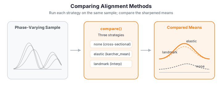
The three aligners each recover a sharp two-peak mean; the constrained method matches the elastic one here because the peaks are the dominant features.

---

What is being compared: distances and warp metrics

To compare methods quantitatively rather than by eye, we need the geometry underneath elastic alignment. It rests on the square-root slope function (SRSF). For an absolutely continuous curve \(f:[0,1]\to\mathbb{R}\),

\[ q(t) \;=\; \operatorname{sgn}\!\big(\dot f(t)\big)\,\sqrt{\,\lvert \dot f(t)\rvert\,}. \]

The point of this transform is that the awkward, non-invariant \(\mathbb{L}^2\) distance between curves becomes the well-behaved Fisher-Rao metric, which the SRSF turns into a plain \(\mathbb{L}^2\) distance. Crucially, under a warp \(\gamma\) (a boundary-preserving diffeomorphism of \([0,1]\), i.e. \(\gamma(0)=0,\ \gamma(1)=1,\ \dot\gamma>0\)), the SRSF transforms by the isometric group action

\[ (q\ast\gamma)(t) \;=\; q\big(\gamma(t)\big)\,\sqrt{\dot\gamma(t)} . \]

Because the action is by isometries, \(\lVert q_1\ast\gamma - q_2\ast\gamma\rVert = \lVert q_1 - q_2\rVert\), and every distance below is invariant to simultaneous rewarping.

Amplitude distance — the residual shape difference after optimal time-warping. It is the Fisher-Rao distance minimized over the warping group \(\Gamma\):

\[ d_a(f_1,f_2) \;=\; \min_{\gamma\in\Gamma}\; \big\lVert\, q_1 \;-\; (q_2\ast\gamma) \,\big\rVert_{\mathbb{L}^2}. \]

This is exactly the objective elastic alignment solves by dynamic programming, so elastic_distance and amplitude_distance coincide (verify below: both return the same value).

Phase distance — the amount of timing difference removed to achieve that match. Warps live on a sphere in SRSF coordinates via \(\psi=\sqrt{\dot\gamma}\) with \(\lVert\psi\rVert=1\), so phase difference is the geodesic (arc) distance on that sphere between the optimal warp \(\gamma^\ast\) and the identity, measured through the Fisher-Rao angle:

\[ d_p(f_1,f_2) \;=\; \cos^{-1}\!\Big(\textstyle\int_0^1 \sqrt{\dot\gamma^\ast(t)}\;dt\Big). \]

Together the pair splits total variation into what the curve looks like (\(d_a\)) and when it happens (\(d_p\)) — the amplitude-phase separation that alignment exists to produce.

Warp complexity — how far a single warp \(\gamma\) departs from doing nothing, again as a Fisher-Rao geodesic distance but now between \(\gamma\) and the identity \(\gamma_{\mathrm{id}}(t)=t\):

\[ c(\gamma) \;=\; d_{FR}(\gamma,\gamma_{\mathrm{id}}) \;=\; \cos^{-1}\!\Big(\textstyle\int_0^1 \sqrt{\dot\gamma(t)}\;dt\Big)\in[0,\tfrac{\pi}{2}). \]

Larger \(c\) means more time-warping was applied; \(c=0\) means the curve was already aligned.

Warp smoothness — the roughness (bending energy) of a warp, penalizing kinks:

\[ s(\gamma) \;=\; \int_0^1 \big(\ddot\gamma(t)\big)^2\,dt . \]

A smooth diffeomorphism has small \(s\); a piecewise-linear landmark warp has \(\ddot\gamma\) concentrated at its kinks, so its bending energy is large — the mechanistic reason landmark and elastic warps look different in the next section.

The figure below computes all four quantities on the phase-varying dataset, each curve measured against the elastic Karcher mean.

import numpy as np
from docs_fig import fig, render
from fdars.alignment import (karcher_mean, amplitude_distance, phase_distance,
                             elastic_distance, warp_complexity, warp_smoothness)

rng = np.random.default_rng(11)
n, m = 14, 150
t = np.linspace(0, 1, m)
base = np.exp(-((t - 0.35) ** 2) / 0.006) + 0.8 * np.exp(-((t - 0.70) ** 2) / 0.006)
data = np.zeros((n, m))
for i in range(n):
    w = t ** rng.uniform(0.7, 1.6)
    data[i] = np.interp(t, (w - w.min()) / np.ptp(w), base)

km = karcher_mean(data, t, max_iter=20)
mu = np.asarray(km["mean"])
gam = np.asarray(km["gammas"])

amp = np.array([amplitude_distance(data[i], mu, t) for i in range(n)])
pha = np.array([phase_distance(data[i], mu, t) for i in range(n)])
cx = np.array([warp_complexity(gam[i], t) for i in range(n)])
sm = np.array([warp_smoothness(gam[i], t) for i in range(n)])

f, axes = fig(ncols=2, figsize=(11, 3.8))
axes[0].scatter(amp, pha, c=cx, cmap="viridis", s=45, edgecolor="k", lw=0.4)
axes[0].set(title="Per-curve split to the elastic mean",
            xlabel=r"amplitude distance $d_a$", ylabel=r"phase distance $d_p$")
cb = f.colorbar(axes[0].collections[0], ax=axes[0])
cb.set_label("warp complexity $c(\\gamma)$", fontsize=8)

axes[1].scatter(cx, sm, color="#6f42c1", s=45, edgecolor="k", lw=0.4)
axes[1].set(title="Warp complexity vs. bending energy",
            xlabel=r"complexity $c(\gamma)$", ylabel=r"smoothness $s(\gamma)$")
print(render(f))

# amplitude distance IS the minimized elastic distance
d_el = np.array([elastic_distance(data[i], mu, t) for i in range(n)])
print(f"max |amplitude_distance - elastic_distance| = {np.abs(amp - d_el).max():.2e}")
print(f"mean phase distance d_p = {pha.mean():.4f} rad "
      f"({np.degrees(pha.mean()):.1f} deg on the warp sphere)")

max |amplitude_distance - elastic_distance| = 0.00e+00 mean phase distance d_p = 0.1392 rad (8.0 deg on the warp sphere)

The left panel shows the amplitude-phase split per curve, coloured by how much warping each needed; curves needing large warps (bright) sit high on the phase axis. The right panel confirms these elastic warps are simultaneously non-trivial (positive complexity) yet smooth (modest bending energy) — the property landmark warps lack. The printout verifies \(d_a\) equals the minimized elastic distance to machine precision.

---

Warping functions: the mechanism differs

The warps expose the fundamental difference. Elastic produces smooth diffeomorphisms; landmark produces piecewise-linear paths kinked at the landmarks; constrained is smooth but passes through the landmark anchors.

import numpy as np
from scipy.signal import find_peaks
from docs_fig import fig, render
from fdars.alignment import karcher_mean, elastic_align_pair_constrained

rng = np.random.default_rng(9)
n, m = 16, 150
t = np.linspace(0, 1, m)
base = np.exp(-((t - 0.35) ** 2) / 0.006) + 0.8 * np.exp(-((t - 0.70) ** 2) / 0.006)
data = np.zeros((n, m))
for i in range(n):
    w = t ** rng.uniform(0.7, 1.5)
    data[i] = np.interp(t, (w - w.min()) / np.ptp(w), base)

# elastic warps
gam_el = np.asarray(karcher_mean(data, t, max_iter=20)["gammas"])

# landmark warps
def top_peaks(y, k, mp=0.2):
    idx, props = find_peaks(y, prominence=mp)
    return np.sort(t[idx[np.argsort(props["prominences"])[::-1][:k]]])
L = np.array([top_peaks(r, 2) for r in data]); target = L.mean(0)
gam_lm = np.array([np.interp(t, np.concatenate(([0.], target, [1.])),
                             np.concatenate(([0.], L[i], [1.]))) for i in range(n)])

# constrained warps
ref = data[0]
gam_c = np.array([np.asarray(elastic_align_pair_constrained(
    ref, data[i], t, target, L[i], lambda_=0.0)["gamma"]) for i in range(n)])

f, axes = fig(ncols=3, figsize=(12, 3.6))
for ax, (g, title, c) in zip(axes, [
        (gam_el, "Elastic (smooth)", "#198754"),
        (gam_lm, "Landmark (kinked)", "#6f42c1"),
        (gam_c, "Constrained (smooth + anchored)", "#0dcaf0")]):
    ax.plot(t, g.T, color=c, lw=1.0, alpha=0.6)
    ax.plot([0, 1], [0, 1], color="#6c757d", ls="--", lw=1.2)
    for x in target:
        ax.axvline(x, color="#adb5bd", ls=":", lw=0.8)
    ax.set(title=title, xlabel="t", aspect="equal")
axes[0].set(ylabel="$\\gamma(t)$")
print(render(f))

The landmark warps have visible corners at the landmark times (dotted verticals); the elastic and constrained warps are smooth, but only the constrained one is pinned to pass through those same times.

---

Quantifying alignment quality

The distances above act per pair; to score a whole method we aggregate. Sharper means come from lower cross-sectional variance, so the headline metric is variance reduction

\[ \mathrm{VR} \;=\; 1-\frac{\overline{\operatorname{Var}}_{\text{aligned}}}{\overline{\operatorname{Var}}_{\text{original}}}, \qquad \overline{\operatorname{Var}} = \frac{1}{m}\sum_{j=1}^{m}\operatorname{Var}_i\!\big(f_i(t_j)\big), \]

the fraction of mean pointwise variance each method removes (\(\mathrm{VR}=1\) is perfect collapse; \(\mathrm{VR}=0\) is no help). We compare all three on two datasets: smooth global phase shifts, and distinct independently-shifting features.

import numpy as np
from scipy.signal import find_peaks
from docs_fig import fig, render
from fdars.alignment import karcher_mean, elastic_align_pair_constrained

t = np.linspace(0, 1, 160)

def make_smooth(seed):
    rng = np.random.default_rng(seed)
    out = np.zeros((15, len(t)))
    for i in range(15):
        s = rng.uniform(-0.1, 0.1); a = rng.normal(1, 0.15)
        out[i] = a * np.sin(2 * np.pi * (t - s)) + 0.4 * a * np.sin(4 * np.pi * (t - 0.7 * s))
    return out

def make_features(seed):
    rng = np.random.default_rng(seed)
    out = np.zeros((15, len(t)))
    for i in range(15):
        p1 = rng.uniform(0.15, 0.35); p2 = rng.uniform(0.55, 0.75)
        out[i] = rng.normal(1, 0.2) * np.exp(-200 * (t - p1) ** 2) + \
                 rng.normal(0.8, 0.15) * np.exp(-200 * (t - p2) ** 2)
    return out

def vr(orig, aligned):
    return 1 - np.var(aligned, axis=0).mean() / np.var(orig, axis=0).mean()

def top_peaks(y, k, mp):
    idx, props = find_peaks(y, prominence=mp)
    if len(idx) == 0:
        return np.array([t[np.argmax(y)]] * k)
    o = np.argsort(props["prominences"])[::-1][:k]
    pk = np.sort(t[idx[o]])
    return np.pad(pk, (0, k - len(pk)), constant_values=pk[-1]) if len(pk) < k else pk

def landmark_align(data, k, mp):
    L = np.array([top_peaks(r, k, mp) for r in data]); target = L.mean(0)
    def reg(y, s):
        kt = np.concatenate(([0.], target, [1.])); ks = np.concatenate(([0.], s, [1.]))
        return np.interp(np.interp(t, kt, ks), t, y)
    return np.array([reg(data[i], L[i]) for i in range(len(data))]), L, target

def constrained_align(data, L, target):
    ref = data[0]
    return np.array([np.asarray(elastic_align_pair_constrained(
        ref, data[i], t, target, L[i], lambda_=0.0)["f_aligned"]) for i in range(len(data))])

results = {}
for name, mk, k, mp in [("smooth", make_smooth, 1, 0.3), ("features", make_features, 2, 0.2)]:
    data = mk(42)
    el = np.asarray(karcher_mean(data, t, max_iter=20)["aligned_data"])
    lm, L, target = landmark_align(data, k, mp)
    cn = constrained_align(data, L, target)
    results[name] = {"Elastic": vr(data, el), "Landmark": vr(data, lm), "Constrained": vr(data, cn)}

methods = ["Elastic", "Landmark", "Constrained"]
x = np.arange(len(methods)); w = 0.38
f, ax = fig()
ax.bar(x - w / 2, [results["smooth"][m] for m in methods], w,
       color="#3f51b5", label="smooth shifts")
ax.bar(x + w / 2, [results["features"][m] for m in methods], w,
       color="#e8710a", label="distinct features")
ax.set(title="Variance reduction by method and dataset",
       ylabel="VR (higher = better)", xticks=x, ylim=(0, 1.05))
ax.set_xticklabels(methods)
ax.legend(fontsize=9)
print(render(f))

for ds in ("smooth", "features"):
    print(ds, {m: round(results[ds][m], 3) for m in methods})

smooth {'Elastic': np.float64(0.582), 'Landmark': np.float64(0.372), 'Constrained': np.float64(0.594)} features {'Elastic': np.float64(0.932), 'Landmark': np.float64(0.829), 'Constrained': np.float64(0.918)}

The pattern mirrors the R reference: on smooth global shifts, elastic and constrained lead and landmark trails (broad oscillations give it few clean anchors); on distinct features, all three do well, with elastic and constrained excellent because the peaks are unambiguous.

Elastic diagnostics

For the elastic method, alignment_quality decomposes the variance and warp_statistics summarizes the warps -- reporting how much work alignment did and how the total splits into amplitude and phase.

import numpy as np
from docs_fig import fig, render
from fdars.alignment import karcher_mean, alignment_quality, warp_statistics

rng = np.random.default_rng(9)
n, m = 16, 140
t = np.linspace(0, 1, m)
base = np.exp(-((t - 0.35) ** 2) / 0.006) + 0.8 * np.exp(-((t - 0.70) ** 2) / 0.006)
data = np.zeros((n, m))
for i in range(n):
    w = t ** rng.uniform(0.7, 1.5)
    data[i] = np.interp(t, (w - w.min()) / np.ptp(w), base)

q = alignment_quality(data, t, lambda_=0.0, max_iter=15)
km = karcher_mean(data, t, max_iter=20)
ws = warp_statistics(np.asarray(km["gammas"]), t, confidence_level=0.95)

f, ax = fig()
labels = ["amplitude\nvariance", "phase\nvariance"]
vals = [float(q["amplitude_variance"]), float(q["phase_variance"])]
ax.bar(labels, vals, color=["#198754", "#6f42c1"])
for i, v in enumerate(vals):
    ax.text(i, v, f"{v:.4f}", ha="center", va="bottom", fontsize=9)
ax.set(title=f"Variance decomposition "
             f"(phase share {float(q['phase_amplitude_ratio']):.0%})",
       ylabel="variance")
print(render(f))

print(f"mean variance reduction : {float(q['mean_variance_reduction']):.4f}")
print(f"phase / amplitude ratio : {float(q['phase_amplitude_ratio']):.4f}")
print(f"mean warp complexity    : {float(q['mean_warp_complexity']):.4f}")
print(f"mean geodesic dist warps: {np.asarray(ws['geodesic_distances']).mean():.4f}")

mean variance reduction : 0.0274 phase / amplitude ratio : 0.9992 mean warp complexity : 0.1121 mean geodesic dist warps: 0.1121

The bar chart splits the total variation into an amplitude part (genuine shape differences) and a phase part (timing), and here the phase bar dominates -- the printed phase/amplitude ratio confirms most of the spread was timing that alignment could remove. The variance-reduction and warp-complexity numbers quantify how much was removed and how hard the warps had to work to do it.

alignment_quality key	Meaning
mean_variance_reduction	Fraction of pointwise variance removed (the VR metric)
total_variance	Total variance before decomposition
amplitude_variance / phase_variance	Variance attributed to amplitude / to phase
phase_amplitude_ratio	Phase share of total -- high means phase-dominated
mean_warp_complexity / mean_warp_smoothness	Average warp magnitude / roughness
pointwise_variance_ratio	Per-point post/pre variance ratio, shape (m,)

A high phase_amplitude_ratio (near 1) confirms the variation is mostly timing -- precisely where alignment helps most.

---

When each method succeeds -- and fails

Real data is messier than tidy examples. These scenarios show where each method shines and where it breaks.

import numpy as np
from scipy.signal import find_peaks
from docs_fig import fig, render
from fdars.alignment import karcher_mean

t = np.linspace(0, 1, 200)

# Scenario A: smooth global warp -- no clean features (elastic wins, landmark struggles)
rng = np.random.default_rng(101)
smooth = np.zeros((12, 200))
for i in range(12):
    ws_ = rng.uniform(-0.15, 0.15)
    tw = t + ws_ * np.sin(np.pi * t)
    tw = (tw - tw.min()) / np.ptp(tw)
    smooth[i] = np.sin(2 * np.pi * tw) + 0.3 * np.cos(6 * np.pi * tw)

# Scenario B: mixed 1-peak & 2-peak curves (elastic handles, landmark forced-template fails)
rng = np.random.default_rng(7)
mixed = np.zeros((12, 200))
for i in range(12):
    if i < 6:
        mixed[i] = 1.5 * np.exp(-300 * (t - rng.uniform(0.3, 0.5)) ** 2)
    else:
        mixed[i] = np.exp(-300 * (t - rng.uniform(0.2, 0.35)) ** 2) + \
                   np.exp(-300 * (t - rng.uniform(0.6, 0.75)) ** 2)

# Scenario C: noisy -- raw vs pre-smoothed elastic
rng = np.random.default_rng(3)
noisy = np.array([np.sin(2 * np.pi * (t - rng.uniform(-0.08, 0.08))) + rng.normal(0, 0.35, 200)
                  for _ in range(12)])
# simple moving-average pre-smoothing
kern = np.ones(11) / 11
smoothed = np.array([np.convolve(y, kern, mode="same") for y in noisy])

el_smooth = np.asarray(karcher_mean(smooth, t, max_iter=20)["aligned_data"])
el_mixed = np.asarray(karcher_mean(mixed, t, max_iter=20)["aligned_data"])
el_noisy_raw = np.asarray(karcher_mean(noisy, t, max_iter=20)["aligned_data"])
el_noisy_sm = np.asarray(karcher_mean(smoothed, t, max_iter=20)["aligned_data"])

f, axes = fig(ncols=3, figsize=(12.5, 3.6))
axes[0].plot(t, el_smooth.T, color="#198754", lw=0.9, alpha=0.5)
axes[0].plot(t, el_smooth.mean(0), color="#e8710a", lw=2.2)
axes[0].set(title="A: smooth warp -> elastic aligns cleanly", xlabel="t", ylabel="f(t)")

axes[1].plot(t, el_mixed.T, color="#3f51b5", lw=0.9, alpha=0.5)
axes[1].plot(t, el_mixed.mean(0), color="#e8710a", lw=2.2)
axes[1].set(title="B: mixed 1-/2-peak -> elastic copes", xlabel="t")

axes[2].plot(t, el_noisy_raw.mean(0), color="#dc3545", lw=2.0, label="raw (over-warps)")
axes[2].plot(t, el_noisy_sm.mean(0), color="#198754", lw=2.0, label="smooth then align")
axes[2].set(title="C: noisy -> smooth first", xlabel="t")
axes[2].legend(fontsize=8)
print(render(f))

Each panel isolates a regime where the method choice matters, and the sharpened orange means show the fix working in every case:

• A -- elastic excels on smooth warping. Broad overlapping oscillations have no clear anchors, so landmark detection has nothing to grab; the Fisher-Rao metric captures the continuous phase change naturally.
• B -- elastic copes with a variable feature count. Half the curves have one peak, half have two. Elastic makes no template assumption; a landmark method with a fixed expected_count=2 would force a spurious second peak onto the single-peak curves.
• C -- smooth before aligning noisy data. The SRSF differentiates the curve, so noise drives over-warping. Pre-smoothing (here a moving average; splines or a kernel smoother work too) or a larger lambda_ tames it.

Scenario summary

Scenario	Best method	Why
Smooth global warping	Elastic	No features to anchor; optimal continuous warp
Independent feature shifts	Landmark	Guarantees feature-to-feature correspondence
Noisy data	Elastic (with lambda_) or pre-smoothing	Penalty / smoothing controls over-warping
Variable number of features	Elastic	No feature template required
Features + smooth variation between them	Constrained elastic	Anchors features and smooths between them

---

Decision guide

	Warping	Automation	Cost	Smoothness	Feature control
Elastic	Smooth diffeomorphism	Fully automatic	\(O(nm^2)\)	High	None
Landmark	Piecewise-linear	Needs feature type	\(O(nm+nk)\)	Low (corners)	Full
Constrained	Smooth with anchors	Needs feature type	\(O(nm^2/k)\)	High between anchors	Partial
TSRVF	(uses elastic)	Fully automatic	\(O(nm^2)\) + PCA	High	None

Situation	Recommended
No prior on which features correspond; smooth timing differences	Elastic (karcher_mean)
Want a principled metric / amplitude-phase decomposition	Elastic + Shape Analysis
Well-defined, domain-meaningful features; need guaranteed correspondence	Landmark (Landmark Registration)
Features must align exactly and the warp between them should be smooth	Constrained (elastic_align_pair_constrained)
PCA / regression / clustering on aligned curves	Elastic + TSRVF

Pitfalls

Method	Common pitfall	Mitigation
Elastic	Over-warping ("pinching") on noisy data	Increase lambda_, or pre-smooth
Landmark	Mismatched landmark correspondence	Use a fixed count, raise the prominence threshold
Constrained	Too few landmarks = barely constrained	Detect more / multiple landmark types
TSRVF	Linearization error for curves far from the mean	Check reconstruction quality

---

A worked workflow

A typical analysis chains the methods: explore, detect features to understand structure, align with the method the structure suggests, then linearize with TSRVF for downstream statistics.

import numpy as np
from scipy.signal import find_peaks
from fdars.alignment import karcher_mean, tsrvf_transform

# 1) explore, 2) understand structure via landmark counts
counts = [len(find_peaks(row, prominence=0.2)[0]) for row in data]
print("peaks per curve:", counts)   # variable count -> prefer elastic

# 3) align (elastic here, since the feature count varies)
km = karcher_mean(data, t, max_iter=15)

# 4) linearize for PCA on the tangent vectors
V = np.asarray(tsrvf_transform(data, t, max_iter=15)["tangent_vectors"])
Vc = V - V.mean(0)
s = np.linalg.svd(Vc, compute_uv=False)
cum = np.cumsum(s ** 2) / np.sum(s ** 2)
print("variance explained (first 3 PCs):", (cum[:3] * 100).round(1))

---

See Elastic Alignment, Advanced Elastic Alignment, Landmark Registration, and TSRVF for the individual methods, and Shape Analysis for the amplitude/phase decomposition that alignment enables.

---

References

The elastic framework, SRSF transform, Fisher-Rao metric, and the amplitude/phase distances used above:

• Srivastava, A. and Klassen, E. P. (2016). Functional and Shape Data Analysis. Springer Series in Statistics. Springer, New York. (Canonical reference for the SRSF, the Fisher-Rao metric, and the amplitude-phase geometry; see Ch. 4-8.)
• Srivastava, A., Wu, W., Kurtek, S., Klassen, E., and Marron, J. S. (2011). Registration of Functional Data Using Fisher-Rao Metric. arXiv:1103.3817. (Introduces the elastic alignment objective \(\min_\gamma \lVert q_1 - (q_2\ast\gamma)\rVert\) and the amplitude/phase separation.)
• Tucker, J. D., Wu, W., and Srivastava, A. (2013). Generative models for functional data using phase and amplitude separation. Computational Statistics & Data Analysis, 61, 50-66. doi:10.1016/j.csda.2012.12.001. (Karcher mean under the elastic metric, variance decomposition, and the alignment-quality diagnostics.)
• Marron, J. S., Ramsay, J. O., Sangalli, L. M., and Srivastava, A. (2015). Functional Data Analysis of Amplitude and Phase Variation. Statistical Science, 30(4), 468-484. doi:10.1214/15-STS524. (Survey contrasting landmark registration with metric-based elastic alignment.)
• Kneip, A. and Gasser, T. (1992). Statistical Tools to Analyze Data Representing a Sample of Curves. The Annals of Statistics, 20(3), 1266-1305. (Foundational treatment of landmark registration and structural averaging.)

fdars companions: vignette("elastic-alignment"), vignette("landmark-registration"), vignette("tsrvf"), and vignette("distance-metrics") in the R package.