Working with Irregular / Sparsely Sampled Functional Data

Textbook functional data arrives as a tidy (n_obs, n_points) matrix: every curve observed at the same grid of points. Real data rarely obliges. Growth studies measure children at whatever ages they happened to visit the clinic; sensors drop samples; longitudinal records are sparse and misaligned. Each curve then lives on its own grid, and the neat matrix disappears.

Irregular sampling shows up almost everywhere functional data does:

Domain	Why the grid is irregular
Longitudinal / clinical studies	patients visited at different times
Sensor networks	dropped packets, varying duty cycles
Environmental monitoring	non-uniform temporal sampling
Financial tick data	trades arrive at irregular intervals

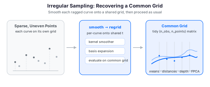
Fdata -- and every pointwise operation built on it (means, distances, depth, FPCA) -- assumes a shared grid. This guide shows why, and how to recover one: smooth each curve onto a common grid with kernel smoothers or a basis expansion, then proceed as usual.

No irregFdata container in fdars (Python)

The R package ships an irregFdata class that stores ragged curves natively (a list of argvals and a list of X), with methods like sparsify(), as.fdata(), is.irregular(), and irregular-aware mean() / metric.lp() / int.simpson(). The Python fdars bindings do not expose that class. Instead we work with plain Python lists of (argvals_i, values_i) pairs and reduce every task to the same move: reconstruct each curve as a smooth function, evaluate all reconstructions on one shared grid, and hand the resulting rectangle to Fdata. Everything below builds that bridge explicitly in NumPy.

Each coloured curve is sampled at a different number of points, at different locations along the domain. There is no shared column to stack these into a matrix, which is precisely why the tidy (n_obs, n_points) layout breaks down and every pointwise operation below needs a common grid first.

---

Why pointwise operations need a common grid

The pointwise mean \(\bar{X}(t) = \frac{1}{n}\sum_i X_i(t)\) is only defined if every \(X_i\) is evaluated at the same \(t\). With curve \(i\) observed at grid \(\{t^{(i)}_1, \dots, t^{(i)}_{m_i}\}\) and curve \(j\) at a different grid, the sum \(X_i(t) + X_j(t)\) has no meaning at a shared column -- the columns do not line up, and \(m_i \neq m_j\) so they cannot even be stacked into a rectangle.

Everything downstream inherits this requirement:

Operation	Why it needs a common grid
Pointwise mean / centering	sums curves column-by-column
\(L^p\) distances / depth	compares \(X_i(t)\) to \(X_j(t)\) at each \(t\)
FPCA	eigen-decomposes a (n_points, n_points) covariance
Basis smoothing of a batch	one (n_obs, n_points) matrix in, one out

The fix is always the same: reconstruct each curve as a smooth function, then evaluate all reconstructions on one shared grid. This is a modelling step, not mere interpolation -- it borrows the smoothness assumption of FDA to fill the gaps between sparse observations.

\[ X_i(t) \;\approx\; \hat{m}_i(t), \qquad \text{then sample } \hat{m}_i \text{ on the common grid } t_1, \dots, t_M . \]

---

Sparsifying regular data (to test a method)

Before trusting a reconstruction on real sparse data, it helps to sparsify a known signal and check how well you recover it. The R package wraps this in sparsify(); in Python it is a two-line helper -- pick a random number of observations per curve, then keep a random subset of the grid:

import numpy as np
from docs_fig import fig, render
from fdars.simulation import simulate

def sparsify(truth, t, min_obs, max_obs, rng, prob=None):
    """Regular (n, len(t)) matrix -> list of (argvals_i, values_i) pairs."""
    curves = []
    for i in range(truth.shape[0]):
        m = int(rng.integers(min_obs, max_obs + 1))
        p = None if prob is None else prob(t) / prob(t).sum()
        idx = np.sort(rng.choice(t.size, size=m, replace=False, p=p))
        curves.append((t[idx], truth[i, idx]))
    return curves

t = np.linspace(0, 1, 200)
truth = np.asarray(simulate(n=12, argvals=t, n_basis=5, seed=42))

# three sampling schemes: uniform, dense-in-middle, dense-at-edges
dense_mid  = lambda s: np.exp(-((s - 0.5) ** 2) / (2 * 0.2 ** 2))
dense_edge = lambda s: 0.1 + 4 * (s - 0.5) ** 2

schemes = {
    "Uniform sampling":  (None, "#3f51b5"),
    "Dense in middle":   (dense_mid, "#e8710a"),
    "Dense at edges":    (dense_edge, "#198754"),
}

f, axes = fig(ncols=3, figsize=(10.5, 3.0))
for ax, (name, (prob, col)) in zip(np.atleast_1d(axes), schemes.items()):
    rng = np.random.default_rng(123)
    for ti, yi in sparsify(truth[:6], t, 15, 25, rng, prob=prob):
        ax.plot(ti, yi, "-", color=col, lw=0.7, alpha=0.35)
        ax.scatter(ti, yi, s=6, color=col, alpha=0.7)
    ax.set(title=name, xlabel="t")
print(render(f))

A non-uniform probability lets you stress-test the parts of the domain a method struggles with: sparse edges expose boundary bias, a sparse middle exposes over-smoothing. We will lean on dense_at_edges later to show why extrapolation matters.

---

Smoothing onto a common grid: kernel smoothers

The kernel smoothers in fdars.smoothing are the natural tool: they take the observed points (x, y) and a target grid x_new, and return the fit at x_new. Because x and x_new are independent, a single call moves a curve from its own sparse grid onto any common grid you choose.

from fdars.smoothing import nadaraya_watson, local_linear, optim_bandwidth

bw = optim_bandwidth(ti, yi)["h_opt"]              # GCV-select on this curve
y_common = nadaraya_watson(ti, yi, common_grid, bandwidth=bw)

Parameter	Type	Description
x	np.ndarray (m,)	the curve's own (irregular) grid
y	np.ndarray (m,)	observed, possibly noisy values
x_new	np.ndarray (M,)	shared target grid for all curves
bandwidth	float	smoothing bandwidth (from optim_bandwidth)
kernel	str	"gaussian", "epanechnikov", "tricube"

Below, one sparse noisy curve is reconstructed on a dense common grid. Note that optim_bandwidth chooses the bandwidth per curve, so sparser curves get more smoothing automatically:

import numpy as np
from docs_fig import fig, render
from fdars.simulation import simulate
from fdars.smoothing import nadaraya_watson, local_linear, optim_bandwidth

t_fine = np.linspace(0, 1, 200)
truth = np.asarray(simulate(n=1, argvals=t_fine, n_basis=5, seed=7))[0]

rng = np.random.default_rng(1)
ti = np.sort(rng.uniform(0, 1, size=22))           # sparse, irregular grid
yi = np.interp(ti, t_fine, truth) + rng.normal(0, 0.15, size=22)

common = np.linspace(0, 1, 200)                     # shared target grid
bw = optim_bandwidth(ti, yi)["h_opt"]
y_nw = np.asarray(nadaraya_watson(ti, yi, common, bandwidth=bw))
y_ll = np.asarray(local_linear(ti, yi, common, bandwidth=bw))

f, ax = fig()
ax.plot(t_fine, truth, color="#198754", lw=2.0, alpha=0.7, label="true signal")
ax.scatter(ti, yi, s=32, color="#6c757d", zorder=3, label="sparse observations")
ax.plot(common, y_nw, color="#3f51b5", lw=2.2, label=f"Nadaraya-Watson (h={bw:.3f})")
ax.plot(common, y_ll, color="#e8710a", lw=2.0, ls="--", label="local linear")
ax.set(title="Sparse points reconstructed on a common grid",
       xlabel="t", ylabel="X(t)")
ax.legend()
print(render(f))

Both smoothers recover the green true signal well through the interior where observations are dense, and the fitted values now live on the 200-point common grid rather than the 22 scattered observations. The two fits diverge mainly near the domain edges, where the sparse one-sided neighbourhood makes reconstruction hardest.

Local linear near the boundaries

On sparse grids the ends of the domain are the weakest spot -- few points to average. local_linear corrects the boundary bias that nadaraya_watson suffers there, so it is usually the safer default for sparse data. See Smoothing for the full comparison.

---

Regridding a whole sample

Once you can move one curve, regridding the sample is a loop that stacks the reconstructions into the (n_obs, M) matrix Fdata wants. After this step the data is rectangular and every pointwise operation is valid again.

import numpy as np
from docs_fig import fig, render
from fdars import Fdata
from fdars.simulation import simulate
from fdars.smoothing import nadaraya_watson, optim_bandwidth

t_fine = np.linspace(0, 1, 200)
truth = np.asarray(simulate(n=20, argvals=t_fine, n_basis=5, seed=7))
rng = np.random.default_rng(3)

common = np.linspace(0, 1, 120)                    # one grid to rule them all
recon = np.empty((truth.shape[0], common.size))
for i in range(truth.shape[0]):
    m = rng.integers(15, 30)                       # each curve: its own sparse grid
    ti = np.sort(rng.uniform(0, 1, size=m))
    yi = np.interp(ti, t_fine, truth[i]) + rng.normal(0, 0.12, size=m)
    bw = optim_bandwidth(ti, yi)["h_opt"]
    recon[i] = nadaraya_watson(ti, yi, common, bandwidth=bw)

fd = Fdata(recon, argvals=common)                  # now a valid Fdata
mu = np.asarray(fd.mean())                         # pointwise mean is defined again

f, ax = fig()
ax.plot(common, recon.T, color="#3f51b5", lw=1, alpha=0.35)
ax.plot(common, mu, color="#e8710a", lw=2.8, label="pointwise mean")
ax.set(title="20 sparse curves regridded, with their mean",
       xlabel="t", ylabel="X(t)")
ax.legend()
print(render(f))

All 20 curves -- each originally on its own ragged grid -- now share the same 120-point axis, so they stack into a rectangle and the pointwise mean (orange) is well-defined again. The regridding loop has rebuilt exactly the tidy structure Fdata needs, and the full functional toolbox is back in play.

Choose the common grid deliberately

A common grid finer than your typical per-curve sampling wastes nothing, but do not extrapolate blindly with a kernel smoother: keep the grid inside the range actually covered by each curve's observations, or the reconstruction at the edges is a guess. A basis fit (next section) can extrapolate sensibly, which is precisely its advantage on truly sparse data.

---

Basis smoothing onto a common grid

Kernel smoothers evaluate wherever you ask, which makes regridding trivial. A basis expansion takes a slightly different route: fdars.basis first fits coefficients on the observed grid, and you then evaluate the same coefficients on the common grid. The two-step pair is:

• fdata_to_basis_1d(y, ti, n_basis, basis_type) -> (coefficients, n_basis) fits a B-spline (or Fourier) expansion to the sparse observations by least squares.
• basis_to_fdata_1d(coefficients, common, n_basis, basis_type) evaluates that expansion on any grid -- here the shared one.

Concretely, with basis functions \(\phi_1, \dots, \phi_K\) the fit solves an ordinary least-squares problem on the observed grid \(t^{(i)}_1, \dots, t^{(i)}_{m_i}\),

\[ \hat{c}_i = \arg\min_{c \in \mathbb{R}^K} \sum_{l=1}^{m_i} \Bigl( y_{il} - \sum_{k=1}^{K} c_k\, \phi_k\bigl(t^{(i)}_l\bigr) \Bigr)^2 , \qquad \hat{x}_i(t) = \sum_{k=1}^{K} \hat{c}_{ik}\, \phi_k(t), \]

and the same coefficients \(\hat{c}_i\) are then evaluated on the common grid. This is the direct analogue of R's fdata2basis() / basis2fdata(), and it is the recommended approach for genuinely sparse data: least squares on the observed points needs no interpolation and handles varying observation densities naturally.

import numpy as np
from docs_fig import fig, render
from fdars.simulation import simulate
from fdars.basis import fdata_to_basis_1d, basis_to_fdata_1d

t_fine = np.linspace(0, 1, 200)
truth = np.asarray(simulate(n=1, argvals=t_fine, n_basis=5, seed=7))[0]

rng = np.random.default_rng(1)
ti = np.sort(rng.uniform(0, 1, size=22))
yi = np.interp(ti, t_fine, truth) + rng.normal(0, 0.15, size=22)

common = np.linspace(0, 1, 200)

# 1. fit coefficients on the sparse, irregular grid
coef, nb = fdata_to_basis_1d(yi[None, :], ti, n_basis=10, basis_type="bspline")
# 2. evaluate the fitted expansion on the common grid
recon = np.asarray(basis_to_fdata_1d(np.asarray(coef), common, nb, basis_type="bspline"))[0]

f, ax = fig()
ax.plot(t_fine, truth, color="#198754", lw=2.0, alpha=0.7, label="true signal")
ax.scatter(ti, yi, s=32, color="#6c757d", zorder=3, label="sparse observations")
ax.plot(common, recon, color="#6f42c1", lw=2.4, label="B-spline reconstruction")
ax.set(title="Basis reconstruction of a sparse curve on a common grid",
       xlabel="t", ylabel="X(t)")
ax.legend()
print(render(f))

For a periodic signal, swap basis_type="fourier" (R's type = "fourier"); the fit and evaluation calls are otherwise identical.

Function	Purpose	Key arguments
fdata_to_basis_1d	fit coefficients to observed points	data, argvals, n_basis, basis_type
basis_to_fdata_1d	evaluate coefficients on a target grid	coefficients, argvals, n_basis, basis_type
pspline_fit_1d	penalized fit at the observed grid	data, argvals, n_basis, lambda_, order
fourier_fit_1d	Fourier fit at the observed grid	data, argvals, nbasis
basis_nbasis_cv	choose n_basis by cross-validation	data, argvals, nbasis_min, nbasis_max, basis_type

pspline_fit_1d / fourier_fit_1d return the fit on the input grid

These convenience fitters return fitted at the same argvals you pass in, so they denoise a curve in place but do not, by themselves, move it to a new grid. To regrid with a penalized fit, take the coefficients they return and feed them to basis_to_fdata_1d on the common grid -- exactly the two-step pattern above.

Direct fitting vs. interpolate-then-fit

Why prefer fitting a basis directly to the sparse points over interpolating onto the common grid first? Because interpolation cannot see past the first and last observation. When a curve's observations do not reach the domain edges -- common under edge-sparse sampling -- linear interpolation leaves NaN there, while a least-squares basis fit extrapolates the trend it has already learned.

import numpy as np
from docs_fig import fig, render
from fdars.simulation import simulate
from fdars.basis import fdata_to_basis_1d, basis_to_fdata_1d

t = np.linspace(0, 1, 100)
truth = np.asarray(simulate(n=1, argvals=t, n_basis=5, seed=42))[0]

# an edge-sparse curve whose observations stop short of the boundaries
rng = np.random.default_rng(11)
inner = (t > 0.12) & (t < 0.86)
idx = np.sort(rng.choice(np.where(inner)[0], size=18, replace=False))
ti, yi = t[idx], truth[idx]

# direct basis fit: extrapolates naturally across the full domain
coef, nb = fdata_to_basis_1d(yi[None, :], ti, n_basis=8, basis_type="bspline")
y_direct = np.asarray(basis_to_fdata_1d(np.asarray(coef), t, nb, basis_type="bspline"))[0]

# interpolate-then-regrid: NaN outside [min(ti), max(ti)]
y_interp = np.interp(t, ti, yi, left=np.nan, right=np.nan)
n_na = int(np.isnan(y_interp).sum())

f, ax = fig()
ax.plot(t, truth, color="#000000", lw=1.6, label="ground truth")
ax.plot(t, y_direct, color="#3f51b5", lw=2.2, ls="--", label="direct basis fit")
ax.plot(t, y_interp, color="#e8710a", lw=2.0, label=f"linear interp ({n_na} NaN)")
ax.scatter(ti, yi, s=28, color="#6c757d", zorder=3, label="observations")
for x in (ti.min(), ti.max()):
    ax.axvline(x, color="#999999", ls=":", lw=1)
ax.set(title="Direct fit spans the full domain; interpolation cannot",
       xlabel="t", ylabel="X(t)")
ax.legend()
print(render(f))

The dotted lines mark the observation range. Inside it both methods agree; only the direct fit produces values in the un-observed margins. With good domain coverage the distinction shrinks, but for truly sparse data direct fitting is the safer default.

P-spline smoothing of noisy curves

When observations are noisy rather than merely sparse, a penalized B-spline (P-spline) trades a small bias for a large variance reduction. pspline_fit_1d takes a roughness penalty lambda_: larger values smooth harder.

import numpy as np
from docs_fig import fig, render
from fdars.simulation import simulate
from fdars.basis import pspline_fit_1d

t = np.linspace(0, 1, 100)
truth = np.asarray(simulate(n=6, argvals=t, n_basis=5, seed=42))
rng = np.random.default_rng(456)
noisy = truth + rng.normal(0, 0.30, size=truth.shape)

# pspline_fit_1d denoises at the SAME grid it is given
res = pspline_fit_1d(noisy, t, n_basis=20, lambda_=0.01)
fitted = np.asarray(res["fitted"] if isinstance(res, dict) else res)

f, (a0, a1) = fig(ncols=2, figsize=(9.5, 3.4))
a0.plot(t, noisy.T, color="#e8710a", lw=0.8, alpha=0.6)
a0.set(title="Noisy data", xlabel="t", ylabel="X(t)")
a1.plot(t, fitted.T, color="#6f42c1", lw=1.4, alpha=0.8)
a1.set(title="P-spline smoothed ($\\lambda=0.01$)", xlabel="t")
print(render(f))

To regrid a P-spline fit rather than denoise in place, pull its coefficients and evaluate them on the common grid with basis_to_fdata_1d, exactly as in the two-step pattern above.

---

Operations once you are back on a common grid

The point of regridding is that the full functional toolbox reopens. A few staples, mirroring the operations the R irregFdata class exposes directly:

Integration and \(L^p\) norms. With any grid in hand, np.trapezoid integrates and fdars.fdata.norm_lp_1d computes \(L^p\) norms. For a constant curve \(c\) on \([0,1]\) the integral is \(c\) and the \(L^2\) norm is \(|c|\) -- a quick sanity check:

import numpy as np
from fdars.fdata import norm_lp_1d

# two constant curves on their own (irregular-length) grids
t1, y1 = np.linspace(0, 1, 50), np.ones(50)
t2, y2 = np.linspace(0, 1, 30), 2 * np.ones(30)

print("<pre>")
print("integral of c=1 :", round(float(np.trapezoid(y1, t1)), 4))
print("integral of c=2 :", round(float(np.trapezoid(y2, t2)), 4))
print("L2 norm  of c=1 :", round(float(np.asarray(norm_lp_1d(y1[None, :], t1, p=2.0))[0]), 4))
print("L2 norm  of c=2 :", round(float(np.asarray(norm_lp_1d(y2[None, :], t2, p=2.0))[0]), 4))
print("</pre>")

integral of c=1 : 1.0
integral of c=2 : 2.0
L2 norm  of c=1 : 1.0
L2 norm  of c=2 : 2.0

Mean estimation: basis vs. kernel. The R vignette estimates the mean of a sparse sample two ways -- a basis reconstruction and a kernel smoother -- and reports the basis mean as far more accurate. In the Python/fdars reproduction the two are much closer, and the kernel mean is in fact marginally better here; see the honest RMSE numbers below. The lesson is the same either way: reconstruct each curve, then average on the common grid.

import numpy as np
from docs_fig import fig, render
from fdars.simulation import simulate
from fdars.smoothing import nadaraya_watson
from fdars.basis import fdata_to_basis_1d, basis_to_fdata_1d

t = np.linspace(0, 1, 100)
truth = np.asarray(simulate(n=50, argvals=t, n_basis=5, seed=42))
rng = np.random.default_rng(123)

recon_b = np.empty((50, t.size))
recon_k = np.empty((50, t.size))
for i in range(50):
    m = int(rng.integers(15, 31))
    idx = np.sort(rng.choice(t.size, size=m, replace=False))
    ti, yi = t[idx], truth[i, idx]
    coef, nb = fdata_to_basis_1d(yi[None, :], ti, n_basis=10, basis_type="bspline")
    recon_b[i] = np.asarray(basis_to_fdata_1d(np.asarray(coef), t, nb, basis_type="bspline"))[0]
    recon_k[i] = np.asarray(nadaraya_watson(ti, yi, t, bandwidth=0.1))

true_mean = truth.mean(axis=0)
mean_b, mean_k = recon_b.mean(axis=0), recon_k.mean(axis=0)
rmse_b = np.sqrt(np.mean((mean_b - true_mean) ** 2))
rmse_k = np.sqrt(np.mean((mean_k - true_mean) ** 2))

f, ax = fig()
ax.plot(t, true_mean, color="#000000", lw=2.2, label="true sample mean")
ax.plot(t, mean_b, color="#3f51b5", lw=1.8, ls="--", label=f"basis mean (RMSE {rmse_b:.4f})")
ax.plot(t, mean_k, color="#e8710a", lw=1.8, ls=":", label=f"kernel mean (RMSE {rmse_k:.4f})")
ax.set(title="Mean of a sparse sample: basis vs. kernel reconstruction",
       xlabel="t", ylabel="mean X(t)")
ax.legend()
print(render(f))

Distance matrix. With curves regridded, any metric in fdars.metric applies. lp_self_1d returns the symmetric pairwise \(L^2\) distance matrix -- the analogue of R's metric.lp() -- ready for clustering or classification:

import numpy as np
from docs_fig import fig, render
from fdars.simulation import simulate
from fdars.metric import lp_self_1d
from fdars.basis import fdata_to_basis_1d, basis_to_fdata_1d

t = np.linspace(0, 1, 100)
truth = np.asarray(simulate(n=5, argvals=t, n_basis=5, seed=42))
rng = np.random.default_rng(123)

recon = np.empty((5, t.size))
for i in range(5):
    idx = np.sort(rng.choice(t.size, size=int(rng.integers(20, 41)), replace=False))
    coef, nb = fdata_to_basis_1d(truth[i, idx][None, :], t[idx], n_basis=10, basis_type="bspline")
    recon[i] = np.asarray(basis_to_fdata_1d(np.asarray(coef), t, nb, basis_type="bspline"))[0]

D = np.asarray(lp_self_1d(recon, t, p=2.0))

f, ax = fig()
im = ax.imshow(D, cmap="viridis")
for (r, c), v in np.ndenumerate(D):
    ax.text(c, r, f"{v:.2f}", ha="center", va="center",
            color="white" if v < D.max() * 0.6 else "black", fontsize=8)
ax.set(title="Pairwise $L^2$ distances (5 regridded curves)",
       xlabel="curve", ylabel="curve")
f.colorbar(im, ax=ax, shrink=0.8)
print(render(f))

The matrix is symmetric with a zero diagonal (each curve is at distance 0 from itself), and the off-diagonal magnitudes rank how dissimilar the regridded curves are -- the raw material any clustering or nearest-neighbour classifier consumes. That such a matrix is computable at all is the whole point of regridding: the distance is only defined once every curve shares one grid.

---

Kernel vs. basis: which to reach for

	Kernel smoothers	Basis expansion
Regrids directly?	yes -- x_new is a free grid	via fdata_to_basis_1d -> basis_to_fdata_1d
Very sparse curves	robust, local_linear fixes edges	needs n_basis below the point count
Extrapolates past observations?	no -- guesses at the edges	yes -- least-squares trend continues
Derivatives afterwards	use local_polynomial(degree=2)	differentiate the basis fit
Periodic data	any kernel	basis_type="fourier"
Cost per curve	one GCV bandwidth search	one linear solve

A practical default: local_linear with a GCV bandwidth for regridding sparse, noisy curves that cover their domain; switch to a B-spline basis when observations do not reach the edges (so you need extrapolation) or when you want coefficients for a downstream model, and to a Fourier basis when the signal is periodic. Use basis_nbasis_cv to pick n_basis rather than guessing.

---

Memory and best practices

Storing only the observed points is far leaner than padding to a dense grid. A regular \(100 \times 1000\) matrix of doubles is \(\approx 781\) KB; the same 100 curves at \(\sim\!50\) observations each (values and argvals) is \(\approx 78\) KB -- an order of magnitude smaller. Since Python fdars has no irregFdata container, you get this saving by keeping your list of (argvals_i, values_i) pairs and only materialising the dense (n_obs, M) matrix at the moment you regrid.

A short preprocessing checklist before regridding:

• Quality control -- drop curves with too few observations to fit your basis (n_basis must be below the point count): [c for c in curves if c[0].size >= 5].
• Domain alignment -- pick a common grid inside the range each curve covers, unless you deliberately want the basis fit to extrapolate.
• Bandwidth / n_basis selection -- use optim_bandwidth or basis_nbasis_cv per curve rather than a single global setting; sparser curves genuinely need more smoothing.

---

References

• Ramsay, J. O. & Silverman, B. W. (2005). Functional Data Analysis (2nd ed.). Springer. (Ch. 4--5, representing and smoothing curves from discrete observations.)
• Yao, F., Müller, H.-G. & Wang, J.-L. (2005). Functional Data Analysis for Sparse Longitudinal Data. Journal of the American Statistical Association, 100(470), 577--590.
• James, G. M., Hastie, T. J. & Sugar, C. A. (2000). Principal Component Models for Sparse Functional Data. Biometrika, 87(3), 587--602.
• Ferraty, F. & Vieu, P. (2006). Nonparametric Functional Data Analysis: Theory and Practice. Springer.

Next Steps

• Smoothing -- the full menu of kernel and basis smoothers, and automatic bandwidth / penalty selection.
• Basis Representation -- what the B-spline and Fourier coefficients mean.
• Custom Plotting -- visualise raw sparse points against the smoothed reconstruction.
• Introduction to fdars -- the Fdata container the common grid feeds into.