Tolerance bands vs conformal bands¶

The problem. Given a sample of curves, draw a band over the whole domain that will contain a stated fraction — say 90% — of curves. fdars offers two routes with different philosophies:

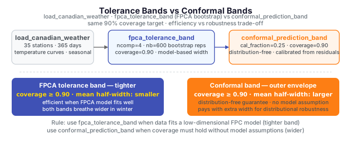
fpca_tolerance_band — model the in-control variation with FPCA and bootstrap the band width. Efficient and tight when the FPCA model fits, but it leans on that model.
conformal_prediction_band — calibrate the width from held-out residuals with no distributional assumptions. Wider and slightly conservative, but the coverage holds whatever the data look like.

This page draws both bands on the same sample of temperature curves and shows the efficiency-vs-robustness trade-off directly.

Tolerance Bands vs Conformal Bands — fpca_tolerance_band FPCA bootstrap vs conformal_prediction_band distribution-free, both at 90% coverage on Canadian weather curves, efficiency vs robustness trade-off

The data¶

Daily temperature for 35 Canadian weather stations — a moderate sample with a clear mean seasonal cycle and heteroscedastic spread (much wider in winter than summer).

import numpy as np
from docs_fig import fig, render
from docs_data import load_canadian_weather

t, temp, meta = load_canadian_weather()

f, ax = fig()
ax.plot(t, temp.T, color="#adb5bd", lw=0.8, alpha=0.5)
ax.set(title="35 temperature curves — the target sample",
       xlabel="day of year", ylabel="temperature (°C)")
print(render(f))

Two bands, one sample¶

Both functions return a band as lower, upper, center and half_width arrays over the domain. Overlaying them at the same 90% target shows the FPCA band hugging the data more tightly while the conformal band sits a little wider.

import numpy as np
from docs_fig import fig, render, fast
from docs_data import load_canadian_weather
from fdars.tolerance import fpca_tolerance_band, conformal_prediction_band

t, temp, meta = load_canadian_weather()
fpca = fpca_tolerance_band(temp, ncomp=4, nb=fast(600, 150), coverage=0.90, seed=1)
conf = conformal_prediction_band(temp, coverage=0.90, seed=1)

f, ax = fig()
ax.plot(t, temp.T, color="#ced4da", lw=0.6, alpha=0.5)
ax.plot(t, fpca["upper"], color="#4A90D9", lw=2, label="FPCA tolerance band")
ax.plot(t, fpca["lower"], color="#4A90D9", lw=2)
ax.plot(t, conf["upper"], color="#E6A020", lw=2, ls="--", label="conformal band")
ax.plot(t, conf["lower"], color="#E6A020", lw=2, ls="--")
ax.set(title="Two 90% bands on the same curves",
       xlabel="day of year", ylabel="temperature (°C)")
ax.legend()
print(render(f))

Both bands breathe with the seasonal heteroscedasticity — narrow in summer, wide in winter — because both are built on functional statistics rather than a constant-width strip. The conformal band (dashed) is the outer envelope.

Efficiency vs robustness¶

The trade-off is quantitative. Empirical coverage is the fraction of curves that stay entirely inside a band; band width is the average half-width across the year.

import numpy as np
from docs_data import load_canadian_weather
from fdars.tolerance import fpca_tolerance_band, conformal_prediction_band

t, temp, meta = load_canadian_weather()
fpca = fpca_tolerance_band(temp, ncomp=4, nb=600, coverage=0.90, seed=1)
conf = conformal_prediction_band(temp, coverage=0.90, seed=1)

def coverage(band):
    lo, up = np.asarray(band["lower"]), np.asarray(band["upper"])
    return np.all((temp >= lo) & (temp <= up), axis=1).mean()

print(f"target coverage: 0.90\n")
print(f"{'band':<14}{'coverage':>10}{'mean half-width':>18}")
print(f"{'FPCA':<14}{coverage(fpca):>10.2f}{np.mean(fpca['half_width']):>18.1f}")
print(f"{'conformal':<14}{coverage(conf):>10.2f}{np.mean(conf['half_width']):>18.1f}")

target coverage: 0.90

band coverage mean half-width FPCA 0.97 22.5 conformal 1.00 27.9

Both reach the target, but the conformal band pays for its distribution-free guarantee with extra width, while the FPCA band is tighter by trusting its low-dimensional model of the variation.

Which to reach for. Use fpca_tolerance_band when the sample is well described by a few principal components and you want the sharpest band; use conformal_prediction_band when you cannot vouch for the model and want coverage you can defend — the same robustness argument as the conformal coverage guarantee for scalar predictions, now lifted to a whole curve.

Parameters¶

Function	Argument	Meaning
`fpca_tolerance_band`	`ncomp`	Number of FPCs modelling the in-control variation
	`nb`	Bootstrap replicates for the width calibration
	`coverage`	Target fraction of curves inside the band
`conformal_prediction_band`	`cal_fraction`	Fraction held out to calibrate the width
	`coverage`	Target coverage `1 − α`

References¶

Degras, D. (2011). Simultaneous confidence bands for nonparametric regression with functional data. Statistica Sinica, 21, 1735–1765.
Lei, J. & Wasserman, L. (2014). Distribution-free prediction bands for non-parametric regression. JRSS-B, 76(1), 71–96.