Functional Boxplot
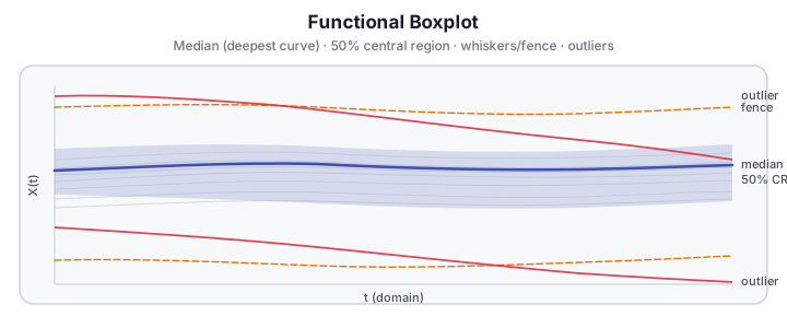
The functional boxplot (López-Pintado & Romo, 2009) is the canonical method for summarising
a sample of curves in the same spirit as Tukey's scalar boxplot: a depth-ranked
median curve, a shaded 50 % central region, whisker/fence lines, and flagged
outlier curves. fdars.depth.functional_boxplot implements this construction
using any of the four depth measures shipped in fdars.depth.
Theory
Functional depth and ranking
Every curve \(X_i\) in the sample is assigned a functional depth score \(D(X_i)\).
A larger score means the curve is more central relative to the sample; a score
near zero means the curve is extreme or peripheral. functional_boxplot supports
four depth measures via the method parameter:
method |
Description |
|---|---|
"fraiman_muniz" |
Pointwise CDF-based depth (Fraiman & Muniz, 2001) |
"band" |
Band depth — proportion of curve inside sample bands |
"modified_band" |
Modified band depth (default); faster, avoids degenerate bands |
"random_projection" |
Projection depth via random half-space projections |
Median
The median is the observed curve with the highest depth score:
It is always an observed sample curve (not a synthetic average).
50 % central region
Rank all \(n\) curves by depth and keep the deepest half. The central region \(C_{0.5}\) is the pointwise envelope of those \(\lceil n/2 \rceil\) most-central curves:
where \(S_{0.5}\) is the index set of the deepest half. The central region plays the role of the interquartile range in a scalar boxplot.
Whiskers / fence
The fence is formed by inflating the central region by factor times its
pointwise width:
The default factor = 1.5 follows the Tukey convention. Sun & Genton (2011)
recommend factor = 1.5 for detecting genuine outliers while avoiding swamping.
Outlier flagging
A curve is an outlier if it exceeds the fence at any evaluation point:
Outlier indices are returned as a Python list of int (0-based row indices).
API
from fdars.depth import functional_boxplot

result = functional_boxplot(data, method="modified_band", factor=1.5)
Parameters
| Parameter | Type | Default | Description |
|---|---|---|---|
data |
ndarray (n, m) |
— | Functional data matrix; rows are observations. Requires \(n \ge 2\). |
method |
str |
"modified_band" |
Depth measure: "fraiman_muniz", "band", "modified_band", or "random_projection". |
factor |
float |
1.5 |
Fence inflation factor (Tukey convention). Must be \(\ge 0\). |
scale |
bool |
True |
Passed to "fraiman_muniz" depth. |
nproj |
int |
50 |
Number of random projection directions for "random_projection". |
seed |
int \| None |
None |
RNG seed for "random_projection" (None resolves to 0). |
Returns — a dict with seven keys:
| Key | Shape | Description |
|---|---|---|
"median" |
(m,) |
The deepest observed curve's values. |
"central_lower" |
(m,) |
Pointwise lower bound of the 50 % central region. |
"central_upper" |
(m,) |
Pointwise upper bound of the 50 % central region. |
"whisker_lower" |
(m,) |
Lower fence: central_lower − factor × width. |
"whisker_upper" |
(m,) |
Upper fence: central_upper + factor × width. |
"outliers" |
Python list[int] |
0-based row indices of curves outside the fence. |
"depths" |
(n,) |
Per-curve depth scores (the ranking used to build the boxplot). |
Worked example
The fence below loads Canadian daily temperature curves (35 stations × 365 days),
downsamples to every other day to keep compute tiny, and runs
functional_boxplot with default settings. It then plots the canonical
López-Pintado–Romo picture and reports the flagged outlier stations.
import numpy as np
from docs_data import load_canadian_weather
from docs_fig import fig, render
from fdars.depth import functional_boxplot

day, X, meta = load_canadian_weather("temperature")
# X: 35 stations × 365 days  → downsample to every other day (183 pts) for speed
X_sub = X[:, ::2]
day_sub = day[::2]

bp = functional_boxplot(X_sub)

median = np.asarray(bp["median"])
cl     = np.asarray(bp["central_lower"])
cu     = np.asarray(bp["central_upper"])
wl     = np.asarray(bp["whisker_lower"])
wu     = np.asarray(bp["whisker_upper"])
out_idx = bp["outliers"]

f, ax = fig(figsize=(10.0, 4.2))

# All curves faint
for i, xi in enumerate(X_sub):
    color = "#dc3545" if i in out_idx else "#adb5bd"
    lw    = 1.8       if i in out_idx else 0.6
    alpha = 0.9       if i in out_idx else 0.35
    ax.plot(day_sub, xi, color=color, lw=lw, alpha=alpha)

# 50 % central region shaded
ax.fill_between(day_sub, cl, cu, color="#3f51b5", alpha=0.18, label="50 % central region")

# Fence lines
ax.plot(day_sub, wu, color="#e8710a", lw=1.4, ls="--", label=f"whisker (factor={1.5})")
ax.plot(day_sub, wl, color="#e8710a", lw=1.4, ls="--")

# Median curve bold
ax.plot(day_sub, median, color="#3f51b5", lw=2.4, label="median (deepest curve)")

ax.set(title="Functional Boxplot — Canadian Weather Temperature",
       xlabel="day of year", ylabel="temperature (°C)")
ax.legend(fontsize=9)
print(render(f))

n_out = len(out_idx)
if n_out:
    names = [meta["station"].iloc[i] for i in out_idx]
    print(f"Flagged outliers ({n_out}): indices {out_idx} → {names}  FDARS_FENCE_OK")
else:
    print(f"Flagged outliers: none at factor=1.5  FDARS_FENCE_OK")
Interpreting the result
Stations flagged as outliers exceed the fence at at least one point in the
year. For Canadian temperatures this typically picks out arctic stations
(very cold winters) or Pacific-coast stations (unusually mild winters).
Increase factor to 2.0 to suppress borderline cases; decrease it to
flag more.
Numeric only — no plot helper yet
functional_boxplot returns the numeric dict. fdars.plot does not yet
ship a plot_functional_boxplot() convenience function. Build your own
figure from the seven keys as shown above.
See also
- Outlier Detection — LRT-based, outliergram, and magnitude-shape outlier detectors.
- Depth Functions — the depth measures
(
fraiman_muniz,band,modified_band,random_projection) used to rank curves in the boxplot.
References
- López-Pintado, S., and Romo, J. (2009). "On the concept of depth for functional data." Journal of the American Statistical Association, 104(486), 718–734. — the depth-fence functional boxplot this page implements.
- Sun, Y., and Genton, M. G. (2011). "Functional boxplots." Journal of
Computational and Graphical Statistics, 20(2), 316–334. — enhanced
functional boxplot with the
factor = 1.5fence convention and visualisation refinements.