TSRVF: Linearized Elastic Analysis

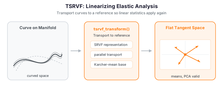
Elastic alignment lives on a curved manifold: the space of functions modulo warping is not a vector space, so ordinary sums, means, and PCA do not apply directly. The Transported Square-Root Velocity Function (TSRVF) representation solves this by parallel-transporting every curve's SRVF to a single reference point -- the Karcher mean -- so that the resulting tangent vectors live in a common linear (Euclidean) space. Once curves are represented as TSRVF tangent vectors, standard linear statistics -- means, covariances, principal components -- become valid again.

The figure below shows a phase-varying sample, its SRSF representation (where the elastic metric becomes the \(L^2\) metric), and the mean SRSF recovered by the TSRVF procedure.

On the left the raw curves are spread by phase; on the right their SRSFs (thin purple) still differ by warping, but the orange mean SRSF \(\mu_q\) recovered by the TSRVF procedure is a clean, un-blurred central shape. That \(\mu_q\) is the base point every curve gets transported to -- the origin of the tangent space in which linear statistics become valid.

---

How it works (intuition)

After elastic alignment the curve shapes live on a curved surface -- the quotient manifold \(\mathcal{F}/\Gamma\). Ordinary statistics assumes flat, Euclidean data, so applying PCA or regression directly distorts the geometry. The TSRVF fixes this by projecting each curve onto a flat tangent plane at the mean shape -- like laying a flat map tangent to the globe at a single point. Near the point of contact the map faithfully approximates the sphere.

Each curve becomes a tangent vector measuring its deviation from the mean shape, and these vectors live in ordinary Euclidean space. That unlocks PCA (to find the dominant modes of shape variation), regression (tangent vectors as predictors), and clustering/classification with any Euclidean method. The projection is invertible, so tangent vectors -- or PC scores, or model predictions -- can be mapped back onto the manifold to reconstruct curves.

---

Concepts

From SRSF to a shared tangent space

The Square-Root Velocity Function (SRVF), also called the SRSF, maps a function \(f\) to

\[ q(t) = \operatorname{sign}\!\big(\dot f(t)\big)\,\sqrt{\lvert \dot f(t)\rvert}. \]

Under this map the Fisher-Rao elastic metric becomes the ordinary \(L^2\) metric, so distances and geodesics can be computed with straightforward \(L^2\) geometry. However, SRVFs of misaligned curves still differ by their warping, so their \(L^2\) average blurs phase structure just like a cross-sectional mean.

The TSRVF construction fixes this in two steps:

1. Align. Compute the Karcher mean \(\mu\) under the elastic metric and the optimal warp \(\gamma_i\) that registers each curve to \(\mu\).
2. Transport. Represent each aligned curve by its SRVF and parallel-transport it to the tangent space at \(\mu_q\) (the mean's SRVF). The transported vectors

$$ v_i \;=\; \log_{\mu_q}!\big(q_i \circ \gamma_i\big) $$

are the tangent vectors returned by the transform. They live in a single Euclidean space \(T_{\mu_q}\), so their sample mean, covariance, and principal components are meaningful.

Because \(v_i\) are ordinary vectors, downstream analysis -- regression on scores, Gaussian modelling, hypothesis tests -- can proceed with classical multivariate tools while still respecting the elastic geometry that generated the data.

The log and exp maps on the sphere

Unit SRSFs live on the Hilbert sphere \(\mathbb{S}^\infty\subset L^2\), where the log map has a closed form. Writing \(\tilde q_i=(q_i\circ\gamma_i)\sqrt{\dot\gamma_i}\) for the aligned SRSF, \(\bar q\) for the mean SRSF, and \(\theta_i=\cos^{-1}\langle\tilde q_i,\bar q\rangle_{L^2}\) for the geodesic angle between them, the tangent vector is

\[ v_i = \log_{\bar q}(\tilde q_i) = \frac{\theta_i}{\sin\theta_i}\,\big(\tilde q_i - \cos\theta_i\,\bar q\big), \]

which is orthogonal to \(\bar q\) and satisfies \(\lVert v_i\rVert_{L^2}=\theta_i\), so tangent-space distances equal geodesic distances exactly at the mean and approximately nearby. The inverse (exponential) map reconstructs the aligned SRSF from any tangent vector \(v\),

\[ \tilde q = \exp_{\bar q}(v) = \cos(\lVert v\rVert)\,\bar q + \sin(\lVert v\rVert)\,\frac{v}{\lVert v\rVert}, \]

and srsf_inverse then turns \(\tilde q\) back into a curve (using the recovered \(f_i(0)\)). This exp map is exactly the reconstruction used in the Inverse transform section below.

Log-map vs. shooting representation

tsrvf_transform_with_method exposes the choice of how curves are mapped into the tangent space. The log_map method uses the Riemannian logarithm at \(\mu_q\) (the default, geometrically exact for the sphere of unit SRSFs); alternative shooting-based representations trade a small amount of fidelity for speed and are useful when only the linear scores matter.

---

Usage

tsrvf_transform(data, argvals, ...) returns the mean, its SRSF, and the transported tangent vectors in one call.

import numpy as np
from fdars.alignment import tsrvf_transform

t = np.linspace(0, 1, 120)
# ... build an (n, m) array `data` of phase-varying curves ...

res = tsrvf_transform(data, t, max_iter=20, tol=1e-4, lambda_=0.0)

V          = res["tangent_vectors"]   # (n, m) -- transported tangent vectors
mu         = res["mean"]              # (m,)   -- Karcher mean function
mu_q       = res["mean_srsf"]         # (m,)   -- mean in SRSF space
srsf_norms = res["srsf_norms"]        # (n,)   -- ||q_i|| for each curve
gammas     = res["gammas"]            # (n, m) -- warps to the mean
converged  = res["converged"]         # bool

Parameter	Type	Description
data	ndarray (n, m)	Sample of \(n\) curves on a common grid
argvals	ndarray (m,)	Evaluation grid (strictly increasing)
max_iter	int	Maximum Karcher-mean iterations (default 20)
tol	float	Convergence tolerance (default 1e-4)
lambda_	float	Warp regularization (default 0.0)

Key	Type	Description
tangent_vectors	ndarray (n, m)	Transported SRVF tangent vectors \(v_i\)
mean	ndarray (m,)	Karcher mean function \(\mu\)
mean_srsf	ndarray (m,)	Mean SRSF \(\mu_q\) (the tangent-space origin)
mean_srsf_norm	float	Norm of the mean SRSF
srsf_norms	ndarray (n,)	SRSF norm of each curve
initial_values	ndarray (n,)	Recovered \(f_i(0)\) (SRSF drops the offset)
gammas	ndarray (n, m)	Optimal warps to the mean
converged	bool	Whether the Karcher mean converged

To select the tangent-space mapping explicitly, use the method variant:

from fdars.alignment import tsrvf_transform_with_method

res = tsrvf_transform_with_method(data, t, method="log_map")   # or a shooting method
V = res["tangent_vectors"]     # same keys as tsrvf_transform

---

Linear statistics in the tangent space

The point of the TSRVF is that the transported vectors behave like ordinary data. Their sample covariance has interpretable eigenvectors, and an SVD of the stacked tangent vectors yields elastic principal components -- a linear PCA that nonetheless respects the warping geometry, because it operates after transport.

import numpy as np
from docs_fig import fig, render
from fdars.alignment import tsrvf_transform

rng = np.random.default_rng(11)
n, m = 24, 120
t = np.linspace(0, 1, m)
base = np.sin(2 * np.pi * t) + 0.5 * np.sin(4 * np.pi * t)
data = np.zeros((n, m))
for i in range(n):
    warp = t ** rng.uniform(0.6, 1.6)
    warp = (warp - warp.min()) / np.ptp(warp)
    data[i] = (1.0 + 0.2 * rng.standard_normal()) * np.interp(t, warp, base)

res = tsrvf_transform(data, t, max_iter=20, tol=1e-4)
V = np.asarray(res["tangent_vectors"])
mu_q = np.asarray(res["mean_srsf"])

# Linear PCA on the transported tangent vectors
Vc = V - V.mean(0)
U, S, Wt = np.linalg.svd(Vc, full_matrices=False)
var_ratio = S**2 / np.sum(S**2)
pc1, pc2 = Wt[0], Wt[1]

f, (a1, a2) = fig(ncols=2, figsize=(9.5, 4.0))
a1.plot(t, mu_q, color="#e8710a", lw=2.2, label="$\\mu_q$")
a1.plot(t, pc1, color="#3f51b5", lw=1.8, label="PC1")
a1.plot(t, pc2, color="#198754", lw=1.8, label="PC2")
a1.set(title="Elastic PCs (tangent space)", xlabel="t", ylabel="component")
a1.legend(fontsize=8)

scores = Vc @ np.vstack([pc1, pc2]).T
a2.scatter(scores[:, 0], scores[:, 1], color="#6f42c1", s=28, alpha=0.8)
a2.set(title=f"Scores (PC1 {var_ratio[0]*100:.0f}%, PC2 {var_ratio[1]*100:.0f}%)",
       xlabel="PC1 score", ylabel="PC2 score")
print(render(f))

The scores are ordinary coordinates: cluster them, regress a response on them, or feed them to a Gaussian model. Because they were computed after transport to \(T_{\mu_q}\), distances between scores approximate elastic distances between the original curves.

Why transport at all?

Averaging SRVFs without alignment reintroduces phase blur. Transport to a common base point is what makes the tangent vectors comparable -- it is the step that turns a curved problem into a flat one.

Visualizing the first mode of variation

Because the tangent space is linear and the exp map is invertible, the leading elastic PC can be turned back into curves: walk along \(\mu_q \pm c\,\mathrm{PC}_1\) in the tangent space, exp-map each point onto the SRSF sphere, and invert with srsf_inverse. The result is a family of curves that shows, in the original data domain, exactly what shape variation PC1 encodes.

import numpy as np
from docs_fig import fig, render
from fdars.alignment import tsrvf_transform, srsf_inverse

rng = np.random.default_rng(11)
n, m = 24, 120
t = np.linspace(0, 1, m)
base = np.sin(2 * np.pi * t) + 0.5 * np.sin(4 * np.pi * t)
data = np.zeros((n, m))
for i in range(n):
    warp = t ** rng.uniform(0.6, 1.6)
    warp = (warp - warp.min()) / np.ptp(warp)
    data[i] = (1.0 + 0.25 * rng.standard_normal()) * np.interp(t, warp, base)

res = tsrvf_transform(data, t, max_iter=20, tol=1e-4)
V = np.asarray(res["tangent_vectors"])
mu_q = np.asarray(res["mean_srsf"])
iv = float(np.asarray(res["initial_values"]).mean())

Vc = V - V.mean(0)
_, S, Wt = np.linalg.svd(Vc, full_matrices=False)
pc1 = Wt[0]
sd1 = S[0] / np.sqrt(len(V))          # score std along PC1

def exp_map(v, mu_q, t):
    norm = np.sqrt(np.trapezoid(v ** 2, t))
    if norm < 1e-9:
        return mu_q.copy()
    return np.cos(norm) * mu_q + np.sin(norm) * (v / norm)

f, ax = fig()
for c, col in [(-1.5, "#3f51b5"), (0.0, "#e8710a"), (1.5, "#198754")]:
    q = exp_map(c * sd1 * pc1, mu_q, t)
    curve = srsf_inverse(q, t, initial_value=iv)
    lab = r"$\mu$" if c == 0 else fr"$\mu {'+' if c > 0 else '-'} {abs(c)}\sigma\,\mathrm{{PC}}_1$"
    ax.plot(t, curve, color=col, lw=2.2 if c == 0 else 1.6, label=lab)
ax.set(title="First elastic mode of variation", xlabel="t", ylabel="f(t)")
ax.legend(fontsize=8)
print(render(f))

The three curves are \(\mu\) and \(\mu \pm 1.5\sigma\) along PC1, all reconstructed through the exp map. They differ mainly in amplitude here -- the dominant shape mode in this sample -- with phase already absorbed by the alignment step. Sweeping the coefficient \(c\) traces a geodesic on the SRSF sphere, so this is a genuine shape interpolation rather than a naive pointwise average.

---

Raw FPCA vs. TSRVF FPCA

The payoff of transport is dimensionality. Standard FPCA on unaligned curves conflates amplitude and phase, so variance spreads across many components. TSRVF FPCA operates on aligned shapes, so the components capture amplitude variation alone -- and the cumulative-variance curve rises faster, needing fewer components for the same coverage.

import numpy as np
from docs_fig import fig, render
from fdars.alignment import tsrvf_transform

rng = np.random.default_rng(42)
n, m = 24, 100
t = np.linspace(0, 1, m)
# amplitude + phase variation on a common shape
data = np.zeros((n, m))
for i in range(n):
    amp = rng.normal(1.0, 0.2)
    shift = rng.uniform(-0.1, 0.1)
    data[i] = amp * np.sin(2 * np.pi * (t - shift))

def cum_var(X):
    Xc = X - X.mean(0)
    s = np.linalg.svd(Xc, compute_uv=False)
    return np.cumsum(s ** 2) / np.sum(s ** 2)

raw = cum_var(data)                                    # FPCA on unaligned curves
V = np.asarray(tsrvf_transform(data, t, max_iter=20, tol=1e-4)["tangent_vectors"])
tsrvf = cum_var(V)                                     # FPCA on tangent vectors

k = np.arange(1, 6)
f, ax = fig()
ax.plot(k, 100 * raw[:5], "o-", color="#6c757d", lw=1.8, label="Raw FPCA")
ax.plot(k, 100 * tsrvf[:5], "o-", color="#3f51b5", lw=1.8, label="TSRVF FPCA")
ax.set(title="Cumulative variance explained", xlabel="number of PCs",
       ylabel="cumulative % variance", ylim=(None, 101))
ax.legend(fontsize=9)
print(render(f))

print(f"PCs to reach 95%  -- raw: {int(np.searchsorted(raw, 0.95)) + 1}, "
      f"TSRVF: {int(np.searchsorted(tsrvf, 0.95)) + 1}")

PCs to reach 95% -- raw: 2, TSRVF: 1

TSRVF FPCA typically needs fewer components: it has already removed phase variation, leaving lower-dimensional amplitude variation behind.

---

Inverse transform (reconstruction)

The transform is invertible -- aligned curves can be rebuilt from their tangent vectors via the exponential map. There is no dedicated tsrvf_inverse binding in the Python surface, but the reconstruction is two transparent lines: apply the exp map to get the aligned SRSF, then srsf_inverse (with the recovered initial value) to get the curve.

import numpy as np
from docs_fig import fig, render
from fdars.alignment import tsrvf_transform, srsf_inverse

rng = np.random.default_rng(4)
n, m = 12, 100
t = np.linspace(0, 1, m)
base = np.sin(2 * np.pi * t) + 0.5 * np.sin(4 * np.pi * t)
data = np.zeros((n, m))
for i in range(n):
    warp = t ** rng.uniform(0.7, 1.5)
    data[i] = np.interp(t, (warp - warp.min()) / np.ptp(warp), base)

res = tsrvf_transform(data, t, max_iter=20, tol=1e-4)
V = np.asarray(res["tangent_vectors"])
mu_q = np.asarray(res["mean_srsf"])
iv = np.asarray(res["initial_values"])

def exp_map(v, mu_q, t):
    norm = np.sqrt(np.trapezoid(v ** 2, t))
    if norm < 1e-9:
        return mu_q.copy()
    return np.cos(norm) * mu_q + np.sin(norm) * (v / norm)

recon = np.array([srsf_inverse(exp_map(V[i], mu_q, t), t, initial_value=float(iv[i]))
                  for i in range(n)])
mu = np.asarray(res["mean"])

f, ax = fig()
ax.plot(t, recon.T, color="#198754", lw=1, alpha=0.5)
ax.plot(t, mu, color="#e8710a", lw=2.4, label="Karcher mean")
ax.set(title="Curves reconstructed from TSRVF tangent vectors",
       xlabel="t", ylabel="f(t)")
ax.legend(fontsize=9)
print(render(f))

Reconstruction from PC scores works the same way: form a tangent vector as mean-plus-a-few-eigenvectors, exp-map it, and invert. This is what lets you synthesize new aligned curves from a fitted low-dimensional model.

Numerical validation: tangent geometry and reconstruction

Two properties the TSRVF construction must satisfy, asserted below on the pure-phase sample above (all curves are warps of one shape, so after alignment they collapse onto the common Karcher mean):

1. Tangent vectors lie in \(T_{\mu_q}\). By construction \(v_i = \log_{\mu_q}(\tilde q_i)\) is orthogonal to the base point \(\mu_q\), i.e. \(\langle v_i, \mu_q\rangle_{\mathbb{L}^2}=0\). This is the exact property that makes linear statistics on the \(v_i\) valid, and it holds to machine precision.
2. Reconstruction recovers the shape. Mapping each \(v_i\) back through the exp map and srsf_inverse reproduces the aligned curve; since the sample is pure phase, every reconstruction lands on the common shape (the Karcher mean) to within a small fraction of the signal amplitude.

max || (tangency): 1.79e-15 (< 1e-10 required) max reconstruction error vs shape / amplitude: 0.038 (< 0.1 required)

Both invariants hold: the tangent vectors are orthogonal to \(\mu_q\) to machine precision (confirming they genuinely live in \(T_{\mu_q}\)), and the exp-map reconstruction lands on the common Karcher mean to within a small fraction of the amplitude. Together these certify that the log/exp round-trip is faithful, so PC scores computed on the \(v_i\) can be safely mapped back to curves.

---

When to use TSRVF

Scenario	Recommended approach
Exploratory alignment & visualization	karcher_mean
PCA on aligned data	tsrvf_transform + SVD (or vert_fpca)
Regression with aligned predictors	tsrvf_transform + standard regression on scores
Clustering aligned curves	tsrvf_transform + any Euclidean clustering
Classification	TSRVF scores as features

The one-liner: TSRVF converts a nonlinear shape-analysis problem into a standard multivariate one, at the cost of a single up-front alignment step.

Relationship to elastic FPCA

tsrvf_transform supplies the transported representation that vertical (amplitude) FPCA operates on. If you want ready-made eigenfunctions and cumulative-variance summaries, use vert_fpca; use the raw tangent vectors here when you need full control over the downstream linear model.

See also Elastic Alignment for the underlying SRSF machinery and Karcher mean, and Shape Analysis for the amplitude/phase decomposition built on this representation.

References

• Srivastava, A., Klassen, E., Joshi, S.H., Jermyn, I.H. (2011). Shape analysis of elastic curves in Euclidean spaces. IEEE TPAMI 33(7):1415-1428.
• Srivastava, A., Klassen, E. (2016). Functional and Shape Data Analysis. Springer. (Exp/log maps on the SRVF sphere.)
• Kurtek, S., Srivastava, A., Klassen, E., Ding, Z. (2012). Statistical modeling of curves using shapes and related features. Journal of the American Statistical Association 107(499):1152-1165.