Cross-Validation for Functional Data
Every functional regression and classifier in fdars has a tuning knob — most often the
number of components \(k\) (FPC, PLS, or shape components). Choosing \(k\) by looking at the
training error is a trap: error falls monotonically as \(k\) grows, so you always pick the
most complex, most over-fit model. Cross-validation breaks this by scoring each model
on data it never saw during fitting, giving an honest estimate of out-of-sample error and
a principled way to select \(k\).
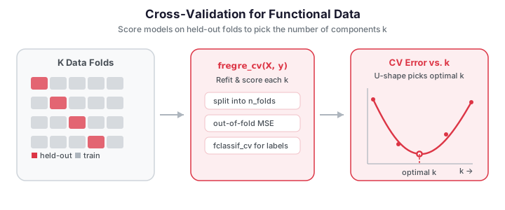
fdars ships dedicated cross-validators — fregre_cv for scalar-on-function regression
and fclassif_cv for functional classification — that do the fold splitting, refitting,
and out-of-fold scoring for you across a grid of component counts.
import numpy as np
from docs_fig import fig, render
from fdars.simulation import simulate
from fdars.regression import fregre_cv

np.random.seed(0)
t = np.linspace(0, 1, 60)
X = np.asarray(simulate(n=40, argvals=t, n_basis=6, efun_type="fourier", seed=1))
beta_true = np.sin(2 * np.pi * t)
y = np.trapezoid(X * beta_true, t, axis=1) + 0.3 * np.random.randn(len(X))

cv = fregre_cv(X, y, k_min=1, k_max=10, n_folds=5)
k = np.asarray(cv["k_values"])
err = np.asarray(cv["cv_errors"])

f, ax = fig()
ax.plot(k, err, "-o", color="#3f51b5", lw=2, ms=6)
ax.axvline(cv["optimal_k"], color="#e8710a", ls="--", lw=1.5,
           label=f"optimal k = {cv['optimal_k']}")
ax.set(title="5-fold CV error vs. number of components",
       xlabel="number of components k", ylabel="CV MSE")
ax.legend()
print(render(f))
The curve has the classic U-shape: too few components under-fit (high bias), too many over-fit (high variance). The minimum marks the sweet spot — often an elbow rather than a sharp valley.
Concepts
In \(K\)-fold cross-validation the sample is partitioned into \(K\) folds. For each fold \(j\), the model is trained on the other \(K-1\) folds and predicts the held-out fold \(j\). The out-of-fold (OOF) predictions \(\hat y_i^{(-j(i))}\) — each made by a model that never saw observation \(i\) — are collected across all folds and scored:
Because every prediction is genuinely out-of-sample, \(\text{CV}(k)\) is an (approximately)
unbiased estimate of test error. Selecting \(\hat k = \arg\min_k \text{CV}(k)\) is model
selection: we search the grid of component counts and keep the one with the lowest honest
error. This is the resampling counterpart to the information criteria in
model_selection_ncomp (GCV/AIC/BIC), which
approximate the same quantity analytically without refitting.
The choice of \(K\) (the number of folds, not components) is itself a bias–variance trade-off:
| \(K\) | Name | Bias of error estimate | Variance | Cost |
|---|---|---|---|---|
| \(n\) | leave-one-out | low | high | \(n\) fits |
| 10 | 10-fold | moderate | moderate | 10 fits |
| 5 | 5-fold | higher | lower | 5 fits |
Five- and ten-fold are the usual defaults: cheap, and stable enough for honest model selection.
Only the number of components is tuned on CV
Cross-validation here selects the number of components. It does not, by
itself, protect against leaking information via preprocessing done on the full
sample before splitting (e.g. centering, scaling, or FPCA on all \(n\) curves).
fregre_cv refits the whole pipeline inside each fold, so its OOF predictions
are clean.
Regression: fregre_cv
import numpy as np
from fdars.simulation import simulate
from fdars.regression import fregre_cv

np.random.seed(0)
t = np.linspace(0, 1, 60)
X = np.asarray(simulate(n=40, argvals=t, n_basis=6, efun_type="fourier", seed=1))
beta_true = np.sin(2 * np.pi * t)
y = np.trapezoid(X * beta_true, t, axis=1) + 0.3 * np.random.randn(len(X))

cv = fregre_cv(X, y, k_min=1, k_max=10, n_folds=5)

print(f"optimal components: {cv['optimal_k']}")
print(f"min CV error:       {cv['min_cv_error']:.4f}")
| Parameter | Type | Description |
|---|---|---|
data |
ndarray (n, m) |
Functional predictors |
response |
ndarray (n,) |
Scalar response |
k_min, k_max |
int |
Range of component counts to search |
n_folds |
int |
Number of CV folds (default 5) |
| Return key | Type | Description |
|---|---|---|
optimal_k |
int |
Component count with lowest CV error |
min_cv_error |
float |
CV MSE at optimal_k |
k_values |
ndarray |
Grid of component counts tested |
cv_errors |
ndarray |
CV MSE for each \(k\) |
oof_predictions |
ndarray (n,) |
Out-of-fold prediction for each observation |
fold_assignments |
ndarray (n,) |
Which fold each observation belongs to |
fold_errors |
ndarray (n_folds,) |
Error contributed by each fold |
The oof_predictions are the honest predictions — plot them against the observed response
to see the model's true generalization, not its optimistic training fit.
Each point is coloured by the fold that predicted it, so no point was used to fit the model that scored it; the cloud hugging the 45-degree line at a healthy OOF \(R^2\) confirms the model generalises rather than merely memorising the training set.
Classification: fclassif_cv
For classifiers, the analogue is the cross-validated misclassification rate. With the same fold structure but a 0/1 loss instead of squared error, the cross-validation objective becomes
the fraction of out-of-fold predictions \(\hat g_i^{(-j(i))}\) whose label disagrees with the
truth \(g_i\). fclassif_cv sweeps the number of components internally and reports the best
count along with the per-fold error.
import numpy as np
from fdars.simulation import simulate
from fdars.classification import fclassif_cv

np.random.seed(1)
t = np.linspace(0, 1, 60)
Xa = np.asarray(simulate(n=20, argvals=t, n_basis=6, efun_type="fourier", seed=1))
Xb = np.asarray(simulate(n=20, argvals=t, n_basis=6, efun_type="fourier", seed=2))
Xa = 0.5 * Xa + np.sin(2 * np.pi * t)            # class 0 mean shape
Xb = 0.5 * Xb + np.sin(2 * np.pi * t) + 1.2 * t  # class 1 mean shape
X = np.vstack([Xa, Xb])
labels = np.r_[np.zeros(20, int), np.ones(20, int)]

cv = fclassif_cv(X, t, labels, method="lda", ncomp=3, nfold=5)

print(f"CV error rate: {cv['error_rate']:.3f}")
print(f"best ncomp:    {cv['best_ncomp']}")
| Parameter | Type | Description |
|---|---|---|
data |
ndarray (n, m) |
Functional predictors |
argvals |
ndarray (m,) |
Evaluation grid |
labels |
ndarray (n,) |
Integer class labels |
method |
str |
Base classifier ("lda", "qda", "knn", …) |
ncomp |
int |
Max number of components to consider |
nfold |
int |
Number of folds |
| Return key | Type | Description |
|---|---|---|
error_rate |
float |
Cross-validated misclassification rate |
fold_errors |
ndarray (nfold,) |
Error rate within each fold |
best_ncomp |
int |
Component count minimizing CV error |
Reading the fold-error spread
A large spread in fold_errors signals an unstable model — the estimate of test error
is itself noisy, often because \(n\) is small relative to the model complexity. Prefer the
simpler model (fewer components) when two settings are within one fold-standard-error of
each other (the "one-standard-error rule").
Comparing methods on shared folds
fregre_cv tunes a single FPC model. To compare different methods fairly, score
them on the same fold split using out-of-fold predictions. fdars has no
single cv.fdata harness (the R package does), but the predict_* functions make
a hand-rolled comparison a few lines:
import numpy as np
from numpy.random import default_rng
from docs_fig import fig, render
from fdars.simulation import simulate
from fdars.regression import predict_fregre_lm, predict_fregre_pls, fregre_np
from fdars.metric import lp_self_1d, lp_cross_1d

np.random.seed(0)
t = np.linspace(0, 1, 60)
X = np.asarray(simulate(n=60, argvals=t, n_basis=6, efun_type="fourier", seed=1))
beta_true = np.sin(2 * np.pi * t)
y = np.trapezoid(X * beta_true, t, axis=1) + 0.3 * np.random.randn(len(X))

def make_folds(n, n_folds, seed):
    return np.array_split(default_rng(seed).permutation(n), n_folds)

def oof(predict, folds):
    out = np.zeros(len(y))
    for f in folds:
        tr = np.setdiff1d(np.arange(len(y)), f)
        out[f] = predict(X[tr], y[tr], X[f])
    return out

def r2(pred):
    return 1 - np.sum((y - pred) ** 2) / np.sum((y - y.mean()) ** 2)

def np_predict(Xtr, ytr, Xte):
    Dtr = lp_self_1d(Xtr, t, p=2.0)
    h = fregre_np(Dtr, ytr, h=0.0)["h_func"]
    Dc = np.asarray(lp_cross_1d(Xte, Xtr, t, p=2.0))
    w = np.exp(-0.5 * (Dc / h) ** 2)
    return (w @ ytr) / w.sum(axis=1)

folds = make_folds(len(y), 5, seed=0)          # SAME folds for every method
methods = {
    "FPC (k=4)": oof(lambda a, b, c: predict_fregre_lm(a, b, c, n_comp=4), folds),
    "PLS (k=4)": oof(lambda a, b, c: predict_fregre_pls(a, t, b, c, n_comp=4), folds),
    "NP (kernel)": oof(np_predict, folds),
}

f, ax = fig()
colors = ["#3f51b5", "#e8710a", "#198754"]
for (name, pred), c in zip(methods.items(), colors):
    ax.scatter(y, pred, s=28, alpha=0.7, color=c, label=f"{name}  R²={r2(pred):.2f}")
lim = [y.min(), y.max()]
ax.plot(lim, lim, color="#6c757d", ls="--", lw=1.5)
ax.set(title="Out-of-fold predictions on shared 5-fold split",
       xlabel="observed y", ylabel="OOF prediction")
ax.legend(fontsize=8)
print(render(f))
Using one fold split for all methods removes split-to-split noise from the comparison — differences in OOF \(R^2\) then reflect the methods, not the shuffle.
Repeated cross-validation
A single \(K\)-fold split is one random partition; its error estimate carries sampling noise. Repeated CV reruns the split with different seeds and averages, and — usefully — exposes per-observation prediction variability. Observations with high spread across repetitions are the fragile ones the model struggles to pin down.
import numpy as np
from numpy.random import default_rng
from docs_fig import fig, render
from fdars.simulation import simulate
from fdars.regression import predict_fregre_lm

np.random.seed(0)
t = np.linspace(0, 1, 60)
X = np.asarray(simulate(n=60, argvals=t, n_basis=6, efun_type="fourier", seed=1))
beta_true = np.sin(2 * np.pi * t)
y = np.trapezoid(X * beta_true, t, axis=1) + 0.3 * np.random.randn(len(X))

def repeated_oof(n_rep=15, n_folds=5):
    preds = np.zeros((n_rep, len(y)))
    for r in range(n_rep):
        folds = np.array_split(default_rng(r).permutation(len(y)), n_folds)
        for fold in folds:
            tr = np.setdiff1d(np.arange(len(y)), fold)
            preds[r, fold] = predict_fregre_lm(X[tr], y[tr], X[fold], n_comp=4)
    return preds

preds = repeated_oof()
mean_pred = preds.mean(0)
sd_pred = preds.std(0)

f, ax = fig()
sc = ax.scatter(y, mean_pred, c=sd_pred, cmap="viridis", s=44)
ax.errorbar(y, mean_pred, yerr=sd_pred, fmt="none",
            ecolor="#adb5bd", alpha=0.6, lw=0.8)
lim = [y.min(), y.max()]
ax.plot(lim, lim, color="#6c757d", ls="--", lw=1.5)
ax.set(title=f"Repeated CV: mean OOF ± SD (mean SD = {sd_pred.mean():.3f})",
       xlabel="observed y", ylabel="mean out-of-fold prediction")
f.colorbar(sc, ax=ax, label="prediction SD")
print(render(f))
The error bars and colour both encode each observation's spread across the 15 repetitions: most points are pinned down tightly, but a handful of high-SD points (brighter, longer bars) are the fragile ones whose prediction flips with the shuffle — exactly the observations to scrutinise before trusting the model on them.
To compare fold splits directly, plotting the per-fold CV error across many repeated splits reveals how much of the reported error is genuine signal versus split-to-split noise:
import numpy as np
from numpy.random import default_rng
from docs_fig import fig, render
from fdars.simulation import simulate
from fdars.regression import predict_fregre_lm

np.random.seed(0)
t = np.linspace(0, 1, 60)
X = np.asarray(simulate(n=60, argvals=t, n_basis=6, efun_type="fourier", seed=1))
beta_true = np.sin(2 * np.pi * t)
y = np.trapezoid(X * beta_true, t, axis=1) + 0.3 * np.random.randn(len(X))

n_rep, n_folds = 30, 5
fold_mse = np.zeros((n_rep, n_folds))
for r in range(n_rep):
    folds = np.array_split(default_rng(r).permutation(len(y)), n_folds)
    for j, fold in enumerate(folds):
        tr = np.setdiff1d(np.arange(len(y)), fold)
        pred = predict_fregre_lm(X[tr], y[tr], X[fold], n_comp=4)
        fold_mse[r, j] = np.mean((y[fold] - pred) ** 2)

overall = fold_mse.mean(1)                       # per-repetition CV estimate

f, ax = fig()
ax.boxplot(fold_mse.T, positions=np.arange(n_rep), widths=0.6,
           showfliers=False, patch_artist=True,
           boxprops=dict(facecolor="#cfd8ff", edgecolor="#3f51b5"),
           medianprops=dict(color="#e8710a"))
ax.plot(np.arange(n_rep), overall, "o", color="#e8710a", ms=4,
        label="per-split CV mean")
ax.axhline(overall.mean(), color="#198754", ls="--", lw=1.5,
           label=f"grand mean = {overall.mean():.3f}")
ax.set(title="Per-fold CV error across 30 repeated 5-fold splits",
       xlabel="repetition", ylabel="fold MSE")
ax.set_xticks([])
ax.legend(fontsize=8)
print(render(f))
Within each repetition the folds scatter widely (the boxes), yet the per-split means (orange) hover close to the green grand mean — a concrete demonstration that a single 5-fold estimate carries real sampling noise, and that averaging over repetitions is what makes the CV error a stable model-selection criterion.
No packaged repeated / nested CV harness in Python
The R reference bundles repeated CV, nested CV, and stratified folds into one
cv.fdata() function. fdars for Python exposes the tuned cross-validators
(fregre_cv, fclassif_cv, and fregre_np_cv for nonparametric-regression
bandwidth selection) plus the predict_* functions; the repeated- and
shared-fold patterns above show how to assemble the rest transparently in a few
lines of numpy. For the kernel method in particular, fregre_np_cv(X, y, argvals,
n_folds=...) packages the bandwidth cross-validation that np_predict above does
by hand — returning the optimal h, the per-bandwidth CV curve, and its SE.
Related pages
- Scalar-on-function regression — the models being tuned, plus
model_selection_ncompfor information-criterion selection. - Regression diagnostics — leave-one-out PRESS, a per-point cousin of CV.
- Conformal prediction — turning honest error into finite-sample coverage guarantees.
References
- Stone, M. (1974). Cross-validatory choice and assessment of statistical predictions. Journal of the Royal Statistical Society: Series B, 36(2), 111–133.
- Allen, D. M. (1974). The relationship between variable selection and data augmentation and a method for prediction. Technometrics, 16(1), 125–127.
- Ramsay, J. O., & Silverman, B. W. (2005). Functional Data Analysis (2nd ed.). Springer.
- Ferraty, F., & Vieu, P. (2006). Nonparametric Functional Data Analysis. Springer.