The conformal coverage guarantee¶

The problem. A regression model predicts the fat content of a meat sample from its near-infrared spectrum, but a single number ŷ = 21.4% says nothing about how much to trust it. We want an interval that contains the true value with a stated probability — and we want that probability to hold without assuming the errors are Gaussian, the model is correct, or anything else about the data-generating process.

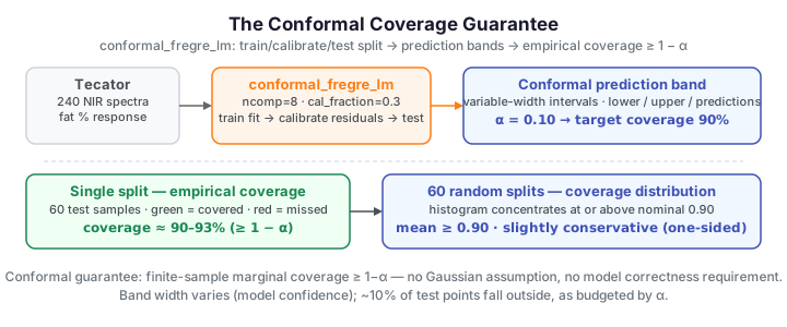
Split conformal prediction delivers exactly that. It wraps any fitted regressor with a calibration step that turns raw residuals into intervals with a finite-sample marginal coverage guarantee: for a miscoverage level \(\alpha\), the interval covers the truth with probability at least \(1-\alpha\). This page demonstrates the guarantee on the Tecator spectra and shows it empirically holding across many random splits.

The Conformal Coverage Guarantee — split conformal prediction on Tecator NIR spectra

The data¶

Tecator records 240 near-infrared absorbance curves (100 wavelengths each); the target is the sample's fat percentage. Spectra of fatty samples sit higher and have a distinctive shoulder — a clean scalar-on-function regression problem.

import numpy as np
from matplotlib import cm
from docs_fig import fig, render
from docs_data import load_tecator

t, X, meta = load_tecator()          # t: (100,), X: (240, 100)
fat = meta["fat"].to_numpy()

f, ax = fig()
norm = (fat - fat.min()) / (fat.max() - fat.min())
for i in np.argsort(fat):
    ax.plot(t, X[i], color=cm.viridis(norm[i]), lw=0.7, alpha=0.7)
ax.set(title="Tecator NIR spectra, coloured by fat content",
       xlabel="wavelength index", ylabel="absorbance")
print(render(f))

Split conformal intervals¶

conformal_fregre_lm fits a functional linear model on a training slice, calibrates on a held-out slice, and returns a lower/upper bound and a point prediction for each test sample. Sorting the test set by prediction shows the intervals as vertical bands; at \(\alpha = 0.1\) we expect about one test point in ten to fall outside its band.

import numpy as np
from docs_fig import fig, render
from docs_data import load_tecator
from fdars.conformal import conformal_fregre_lm

t, X, meta = load_tecator()
y = meta["fat"].to_numpy()

rng = np.random.default_rng(0)
idx = rng.permutation(len(y))
test, train = idx[:60], idx[60:]
res = conformal_fregre_lm(X[train], y[train], X[test],
                          ncomp=8, cal_fraction=0.3, alpha=0.1, seed=1)
lo, up, pred = res["lower"], res["upper"], res["predictions"]
truth = y[test]
covered = (truth >= lo) & (truth <= up)

o = np.argsort(pred)                      # sort by prediction for a readable chart
xs = np.arange(len(o))
f, ax = fig()
ax.vlines(xs, lo[o], up[o], color="#adb5bd", lw=2)
ax.scatter(xs[covered[o]], truth[o][covered[o]], color="#2E8B57", s=18, label="covered")
ax.scatter(xs[~covered[o]], truth[o][~covered[o]], color="#D55E00", s=24, label="missed")
ax.set(title=f"90% conformal intervals — empirical coverage {covered.mean():.0%}",
       xlabel="test sample (sorted by prediction)", ylabel="fat (%)")
ax.legend()
print(render(f))

Almost every truth (green) sits inside its band; the handful of red misses is exactly the ~10% miscoverage the level \(\alpha = 0.1\) budgets for. Note the bands are not all the same width — that is the model expressing where it is more or less certain.

The guarantee holds across splits¶

A single split could get lucky. The guarantee is about the long run: repeat the train/calibrate/test split many times and the empirical coverage concentrates around the nominal \(1-\alpha = 0.90\), regardless of which samples happen to land where.

import numpy as np
from docs_fig import fig, render, fast
from docs_data import load_tecator
from fdars.conformal import conformal_fregre_lm

t, X, meta = load_tecator()
y = meta["fat"].to_numpy()
n = len(y)

n_splits = fast(60, 12)                   # full build: 60 splits; DOCS_FAST: 12
covs = []
for s in range(n_splits):
    idx = np.random.default_rng(s).permutation(n)
    test, train = idx[:60], idx[60:]
    r = conformal_fregre_lm(X[train], y[train], X[test],
                            ncomp=8, cal_fraction=0.3, alpha=0.1, seed=s)
    covs.append(((y[test] >= r["lower"]) & (y[test] <= r["upper"])).mean())
covs = np.array(covs)

f, ax = fig()
ax.hist(covs, bins=12, color="#4A90D9", alpha=0.8, edgecolor="white")
ax.axvline(0.90, color="#D55E00", lw=2, ls="--", label="nominal 1 − α = 0.90")
ax.axvline(covs.mean(), color="#2E8B57", lw=2, label=f"mean = {covs.mean():.2f}")
ax.set(title=f"Empirical coverage over {n_splits} random splits",
       xlabel="coverage", ylabel="count")
ax.legend()
print(render(f))

The distribution sits on or just above the dashed nominal line: conformal prediction is (slightly) conservative, never systematically under-covering. That one-sided robustness — coverage you can rely on without distributional assumptions — is why conformal intervals are the honest way to quantify uncertainty for a black-box functional regressor.

Parameters¶

Argument	Default	Meaning
`ncomp`	`3`	Number of functional principal components the linear model uses
`cal_fraction`	`0.25`	Fraction of the training data held out to calibrate the interval width
`alpha`	`0.1`	Miscoverage level; the interval targets coverage `1 − alpha`
`seed`	`42`	RNG seed for the calibration split

References¶

Vovk, V., Gammerman, A. & Shafer, G. (2005). Algorithmic Learning in a Random World. Springer.
Lei, J., G'Sell, M., Rinaldo, A., Tibshirani, R. & Wasserman, L. (2018). Distribution-free predictive inference for regression. JASA, 113(523), 1094–1111.