Elastic Clustering

Two curves can have the same shape yet look far apart under the ordinary \(L^2\) metric simply because their features are shifted in time -- a peak at \(t=0.4\) versus the same peak at \(t=0.6\). Standard clustering (k-means, GMM) inherits this weakness: it groups by pointwise value, so phase variation masquerades as amplitude variation and the recovered clusters track alignment rather than true shape.

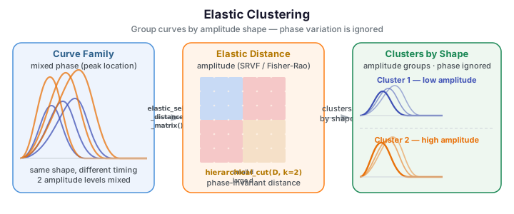
Elastic clustering removes phase before comparing curves. It measures dissimilarity with an amplitude (elastic) distance -- a metric on the Fisher--Rao geometry of curves that is invariant to monotone time-warping -- and then clusters the resulting distance matrix. fdars.alignment provides the elastic distance matrices and distance-based clusterers needed for this pipeline.

import numpy as np
from docs_fig import fig, render
from fdars.alignment import elastic_self_distance_matrix, hierarchical_cut

# Two AMPLITUDE groups (peak height 1 vs 2); each curve has a RANDOM peak
# location, so phase is pure nuisance variation.
t = np.linspace(0, 1, 60)
rng = np.random.default_rng(4)
def bump(c, h, w=0.006):
    return h * np.exp(-((t - c) ** 2) / (2 * w))
X, true = [], []
for gi, h in enumerate([1.0, 2.0]):
    for _ in range(15):
        c = rng.uniform(0.25, 0.75)                 # random phase
        X.append(bump(c, h) + 0.02 * rng.standard_normal(len(t)))
        true.append(gi)
X = np.asarray(X)

D = elastic_self_distance_matrix(X, t)              # phase-invariant distances
labels = np.asarray(hierarchical_cut(D, k=2, linkage="average"))
palette = ["#3f51b5", "#e8710a"]

f, ax = fig()
for xi, li in zip(X, labels):
    ax.plot(t, xi, color=palette[li], lw=1.0, alpha=0.6)
ax.set(title="Curves colored by elastic cluster (peak height, not location)",
       xlabel="t", ylabel="X(t)")
print(render(f))

The clusters split the curves by peak height -- the true amplitude groups -- and ignore where each peak happens to sit.

---

Concepts

The square-root velocity representation

Elastic distances are computed in the square-root velocity function (SRVF) representation. For a curve \(f\) with derivative \(\dot f\), its SRVF is

\[ q(t) \;=\; \operatorname{sign}\!\bigl(\dot f(t)\bigr)\,\sqrt{|\dot f(t)|}. \]

Under this transform, warping the time axis of \(f\) by a monotone reparameterisation \(\gamma\) acts on \(q\) by the norm-preserving action \((q, \gamma) \mapsto (q \circ \gamma)\sqrt{\dot\gamma}\). The amplitude (elastic) distance between \(f_1\) and \(f_2\) optimises over all warps,

\[ d_A(f_1, f_2) \;=\; \min_{\gamma \in \Gamma} \bigl\| q_1 - (q_2 \circ \gamma)\sqrt{\dot\gamma} \,\bigr\|_2 , \]

so two curves that differ only by time-warping have distance \(0\). This is exactly the invariance that fools \(L^2\): under \(d_A\), phase-shifted copies of a shape collapse to a single point.

fdars.alignment exposes three self-distance matrices built on this geometry:

Function	Distance	Invariant to
elastic_self_distance_matrix	amplitude (elastic)	monotone time-warping
amplitude_self_distance_matrix	amplitude (alias of the above)	monotone time-warping
shape_self_distance_matrix	shape	warping and a chosen quotient (e.g. reparameterisation)

Each returns a symmetric \((n, n)\) matrix with a zero diagonal, ready to feed to a distance-based clusterer.

Why \(L^2\) k-means fails here

\(L^2\) k-means compares curves value-by-value. When peaks are shifted, two curves from the same amplitude group can be nearly disjoint (peak of one aligns with the baseline of the other), inflating their \(L^2\) distance above that of curves from different amplitude groups whose peaks happen to overlap. The partition then reflects peak location rather than the amplitude structure we care about.

elastic purity = 1.000 L2 k-means purity = 0.567 (elastic beats L2 by 0.433)

Elastic clustering recovers the amplitude groups almost perfectly (asserted purity \(\ge 0.95\)), while \(L^2\) k-means -- distracted by phase -- lands close to a coin flip. The two asserts above make this a checked claim: the elastic partition matches the known amplitude labels and beats \(L^2\) by a wide margin, not merely by eye.

---

Clustering a distance matrix

Once the elastic distance matrix is in hand, any distance-based clusterer applies. fdars.alignment ships two.

hierarchical_cut

A convenience wrapper that runs agglomerative clustering and cuts the tree to \(k\) groups.

from fdars.alignment import elastic_self_distance_matrix, hierarchical_cut

D = elastic_self_distance_matrix(X, t)
labels = hierarchical_cut(D, k=2, linkage="average")   # -> (n,) int labels

Parameter	Type	Default	Description
dist_mat	ndarray (n, n)	--	Precomputed distance matrix
k	int	2	Number of clusters to cut to
linkage	str	"single"	Linkage rule ("single", "average", ...)

Returns an (n,) integer label vector. The related hierarchical_from_distances(dist_mat, linkage=...) returns the full merge sequence as a dict with keys merges and n if you need the tree itself.

kmedoids_from_distances

K-medoids picks actual curves as cluster centres (medoids), which is natural when only pairwise distances -- not coordinates -- are available.

from fdars.alignment import kmedoids_from_distances

km = kmedoids_from_distances(D, k=2, seed=1)
labels  = km["labels"]           # (n,) int
medoids = km["medoid_indices"]   # (k,) indices of representative curves

Parameter	Type	Default	Description
dist_mat	ndarray (n, n)	--	Precomputed distance matrix
k	int	2	Number of clusters
max_iter	int	100	Maximum iterations
seed	int	42	Random seed

Returns a dictionary with keys labels, medoid_indices, within_distances, total_within_distance, n_iter and converged.

---

Reading the distance matrix

Reordering the elastic distance matrix so that curves in the same cluster are adjacent reveals a clear block structure: small (dark) within-cluster distances on the diagonal blocks, large (bright) between-cluster distances off-diagonal. This is a quick visual check that the clusters are real rather than an artefact of the cut.

The two dark diagonal blocks are the amplitude groups; the bright off-diagonal blocks separate them.

Amplitude vs. shape distance

Use elastic_self_distance_matrix / amplitude_self_distance_matrix when you want to cluster by amplitude with phase removed. Use shape_self_distance_matrix (with a quotient, e.g. "reparameterization") when even the overall scale or a further group action should be quotiented out and only pure shape should drive the clusters.

Cost

Elastic distances solve a warping optimisation for every pair, so building the \((n, n)\) matrix is \(\mathcal{O}(n^2)\) alignments. Keep \(n\) modest (tens to low hundreds), or precompute the matrix once and reuse it across hierarchical_cut, kmedoids_from_distances and the cluster-quality indices.

---

Choosing the number of clusters

When the number of groups is unknown, sweep \(k\) and plot the total within-cluster distance from kmedoids_from_distances (total_within_distance). A sharp drop followed by a plateau -- the elbow -- flags the natural number of clusters. On the two-amplitude example the distance falls steeply from \(k=1\) to \(k=2\) and then flattens, correctly pointing at two groups.

import numpy as np
from docs_fig import fig, render
from fdars.alignment import elastic_self_distance_matrix, kmedoids_from_distances

t = np.linspace(0, 1, 60)
rng = np.random.default_rng(4)
def bump(c, h, w=0.006):
    return h * np.exp(-((t - c) ** 2) / (2 * w))
X = []
for h in [1.0, 2.0]:
    for _ in range(15):
        c = rng.uniform(0.25, 0.75)
        X.append(bump(c, h) + 0.02 * rng.standard_normal(len(t)))
X = np.asarray(X)

D = np.asarray(elastic_self_distance_matrix(X, t))
ks = list(range(1, 7))
twd = [float(kmedoids_from_distances(D, k=k, seed=1)["total_within_distance"]) for k in ks]

f, ax = fig(figsize=(7.0, 3.6))
ax.plot(ks, twd, "-o", color="#3f51b5", lw=1.8)
ax.axvline(2, color="#e8710a", ls="--", lw=1.2, label="elbow at k = 2")
ax.set(title="Elastic k-medoids: total within-cluster distance vs. k",
       xlabel="k", ylabel="total within-cluster distance")
ax.legend()
print(render(f))

The total within-cluster distance drops sharply from \(k = 1\) to \(k = 2\) and then flattens, so the elbow lands at \(k = 2\) -- exactly the two amplitude groups built into the data, recovered without any knowledge of the peak locations.

Reading off the medoid prototypes

Because k-medoids picks actual curves as centres, the medoid_indices it returns are representative exemplars you can plot directly. For the two-amplitude example the two medoids should be a low-peak curve and a high-peak curve -- the archetypes of each group, regardless of where their peaks happen to fall.

import numpy as np
from docs_fig import fig, render
from fdars.alignment import elastic_self_distance_matrix, kmedoids_from_distances

t = np.linspace(0, 1, 60)
rng = np.random.default_rng(4)
def bump(c, h, w=0.006):
    return h * np.exp(-((t - c) ** 2) / (2 * w))
X = []
for h in [1.0, 2.0]:
    for _ in range(15):
        c = rng.uniform(0.25, 0.75)
        X.append(bump(c, h) + 0.02 * rng.standard_normal(len(t)))
X = np.asarray(X)

D = np.asarray(elastic_self_distance_matrix(X, t))
km = kmedoids_from_distances(D, k=2, seed=1)
labels = np.asarray(km["labels"])
medoids = np.asarray(km["medoid_indices"])
palette = ["#3f51b5", "#e8710a"]

f, ax = fig()
for xi, li in zip(X, labels):
    ax.plot(t, xi, color=palette[li], lw=0.7, alpha=0.25)
for k, mi in enumerate(medoids):
    ax.plot(t, X[mi], color=palette[k], lw=2.8, label=f"medoid of cluster {k}")
ax.set(title="K-medoids prototypes (bold) over their clusters",
       xlabel="t", ylabel="X(t)")
ax.legend()
print(render(f))

The two bold medoid curves capture the essential contrast -- one low peak, one high peak -- while their differing peak positions confirm that k-medoids selected exemplars on amplitude, treating the phase of each prototype as incidental.

Elbows on elastic distances can be gentle

Because alignment already collapses phase variation, the within-distance curve is often smoother than for \(L^2\) clustering -- the elbow is a nudge, not a cliff. Read it alongside the reordered distance-matrix heatmap above and, where you have labels, a purity or silhouette check on the elastic distances.

---

Related pages

• Clustering -- \(L^2\) k-means, fuzzy c-means, GMM and quality indices.
• Model-based clustering -- soft assignments via Gaussian mixtures.
• fdars.alignment -- elastic alignment, Karcher means and the SRVF machinery behind these distances.

References

• Srivastava, A., Klassen, E. (2016). Functional and Shape Data Analysis. Springer.
• Tucker, J.D., Wu, W., Srivastava, A. (2013). Generative Models for Functional Data Using Phase and Amplitude Separation. Computational Statistics & Data Analysis, 61, 50–66.
• Kurtek, S., Srivastava, A., Klassen, E., Ding, Z. (2012). Statistical Modeling of Curves Using Shapes and Related Features. Journal of the American Statistical Association, 107(499), 1152–1165.