Ranking curves by centrality with functional depth¶

The problem. Given a sample of curves, which ones are typical and which are atypical? For scalars we would reach for the median and the quartiles, but a curve has no natural ordering — you cannot sort 35 temperature trajectories from "smallest" to "largest". Functional depth supplies the missing order: it scores each curve by how central it sits within the sample, so the deepest curve is a functional median and the shallowest curves are candidate outliers.

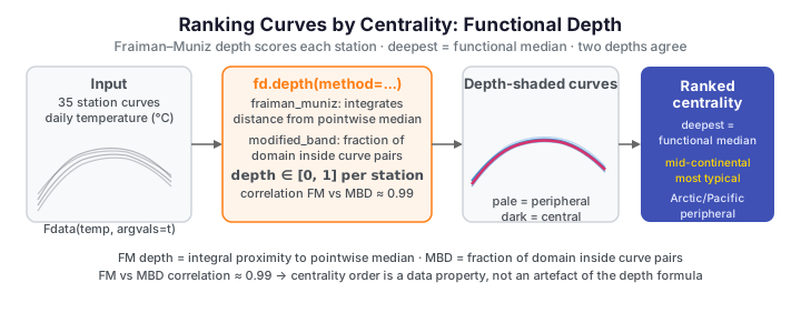
This page ranks the daily temperature curves of 35 Canadian weather stations by depth, reads off the most and least typical climates, and shows that two different depth notions produce essentially the same ordering.

Ranking Curves by Centrality with Functional Depth — Fraiman-Muniz and modified band depth ordering

The data¶

Each station contributes one curve: daily temperature across the year. Plotted together they form a band a few degrees wide in summer that fans out over the cold months.

import numpy as np
from docs_fig import fig, render
from docs_data import load_canadian_weather

t, temp, meta = load_canadian_weather()   # t: (365,), temp: (35, 365)

f, ax = fig()
ax.plot(t, temp.T, color="#6c757d", lw=0.8, alpha=0.4)
ax.set(title="Daily temperature — 35 Canadian weather stations",
       xlabel="day of year", ylabel="temperature (°C)")
print(render(f))

The winter spread is what makes a single "average curve" unsatisfying: a pointwise mean runs through the middle of the band but corresponds to no real station, and it says nothing about which stations are representative of the group.

Ranking by depth¶

Wrap the curves in an Fdata object and call depth(). The default Fraiman–Muniz depth integrates, at every day of the year, how far each curve sits from the pointwise median; a curve that stays near the centre all year scores high.

import numpy as np
from matplotlib import cm
from docs_fig import fig, render
from docs_data import load_canadian_weather
from fdars import Fdata

t, temp, meta = load_canadian_weather()
fd = Fdata(temp, argvals=t)
depth = fd.depth(method="fraiman_muniz")        # (35,) in [0, 1]

# shade each curve by its depth: pale = peripheral, dark = central
norm = (depth - depth.min()) / (depth.max() - depth.min())
f, ax = fig()
for i in np.argsort(depth):                      # draw shallow first, deep on top
    ax.plot(t, temp[i], color=cm.Blues(0.25 + 0.75 * norm[i]), lw=1.0)
deepest = int(np.argmax(depth))
ax.plot(t, temp[deepest], color="#d6336c", lw=2.5, label="deepest (functional median)")
ax.set(title="Temperature curves shaded by Fraiman–Muniz depth",
       xlabel="day of year", ylabel="temperature (°C)")
ax.legend()
print(render(f))

The dark curves cluster in the centre of the band; the pale ones are the extreme climates that ride its upper and lower edges. The highlighted red curve is the deepest station — the closest thing the sample has to a median climate, and unlike the pointwise mean it is an actual observed station.

The most and least typical climates¶

Sorting by depth turns the picture into a ranked list. The central stations are mid-continental; the peripheral ones are the maritime and far-north extremes.

import numpy as np
from docs_data import load_canadian_weather
from fdars import Fdata

t, temp, meta = load_canadian_weather()
depth = Fdata(temp, argvals=t).depth(method="fraiman_muniz")
order = np.argsort(depth)[::-1]                  # deepest first

print("Most central (typical climate):")
for i in order[:3]:
    r = meta.iloc[i]
    print(f"  {r['station']:<15} {r['province']:<8} {r['region']:<12} depth={depth[i]:.3f}")

print("\nMost peripheral (atypical climate):")
for i in order[-3:][::-1]:
    r = meta.iloc[i]
    print(f"  {r['station']:<15} {r['province']:<8} {r['region']:<12} depth={depth[i]:.3f}")

Most central (typical climate): Thunder Bay Ontario Continental depth=0.868 Bagottville Quebec Atlantic depth=0.807 Sherbrooke Quebec Atlantic depth=0.796

Most peripheral (atypical climate): Resolute Nunavut Arctic depth=0.058 Iqaluit Nunavut Arctic depth=0.184 Kamloops British Colombia Pacific depth=0.188

The interpretation is geographic: a deep curve belongs to a station whose seasonal cycle is representative of the country as a whole, while a shallow curve flags a station whose climate is unusual — exactly the ranking you would want before fitting a model that assumes the sample is homogeneous.

Different depth notions, same ordering¶

"Depth" is not a single formula. Modified band depth (MBD) scores a curve by the fraction of the domain on which it lies inside the band traced by pairs of other curves — a completely different construction from Fraiman–Muniz. Reassuringly, on this sample the two rankings agree almost perfectly, so the centrality ordering is a property of the data rather than an artefact of one particular depth.

import numpy as np
from docs_fig import fig, render
from docs_data import load_canadian_weather
from fdars import Fdata

t, temp, meta = load_canadian_weather()
fd = Fdata(temp, argvals=t)
fm  = fd.depth(method="fraiman_muniz")
mbd = fd.depth(method="modified_band")
rho = np.corrcoef(fm, mbd)[0, 1]

f, ax = fig()
ax.scatter(fm, mbd, color="#3f51b5", s=30)
ax.set(title=f"Two depth notions agree (correlation = {rho:.2f})",
       xlabel="Fraiman–Muniz depth", ylabel="Modified band depth")
print(render(f))

When two independent depths disagree it is usually a sign of multimodality — several distinct groups of curves, each central to its own cluster. Here the tight diagonal says the stations form one coherent population with a clear centre-to-edge gradient.

Parameters¶

Argument	Default	Meaning
`method`	`"fraiman_muniz"`	Depth definition — also `"modified_band"`, `"band"`, `"modal"`, `"random_projection"`, `"random_tukey"`, and more
`ref`	`None`	Optional reference `Fdata` to measure depth against (e.g. score new curves relative to a training sample); defaults to the sample itself

References¶

Fraiman, R. & Muniz, G. (2001). Trimmed means for functional data. Test, 10(2), 419–440.
López-Pintado, S. & Romo, J. (2009). On the concept of depth for functional data. JASA, 104(486), 718–734.